class: center, top, title-slide .title[ # <strong>Exponential Growth Part III: Randomness and Stochasticity</strong> ] .subtitle[ ## <a href="https://eligurarie.github.io/EFB370/">EFB 370: Population Ecology</a> ] .author[ ### <strong>Dr. Elie Gurarie</strong> ] .date[ ### <strong>February 19, 2024</strong> ] --- class:inverse <!-- https://bookdown.org/yihui/rmarkdown/xaringan-format.html --> .pull-left.large[ ## Goals (concepts / buzzwords) - **I. Random variables:** - mean / variance / standard deviation / distributions / expected value - Binomial and Normal distributions - II **stochastic** = randomness in time - **demographic stochasticity** = randomness in individual processes - **environmental stochasticity** = randomness affecting populations ] .pull-right.large[ ### Suggested reading: - Gotelli: Chapter 1 (second half) ] --- ## If the exponential model is so tidy ... why isn't it *perfect*? .pull-left-50[ 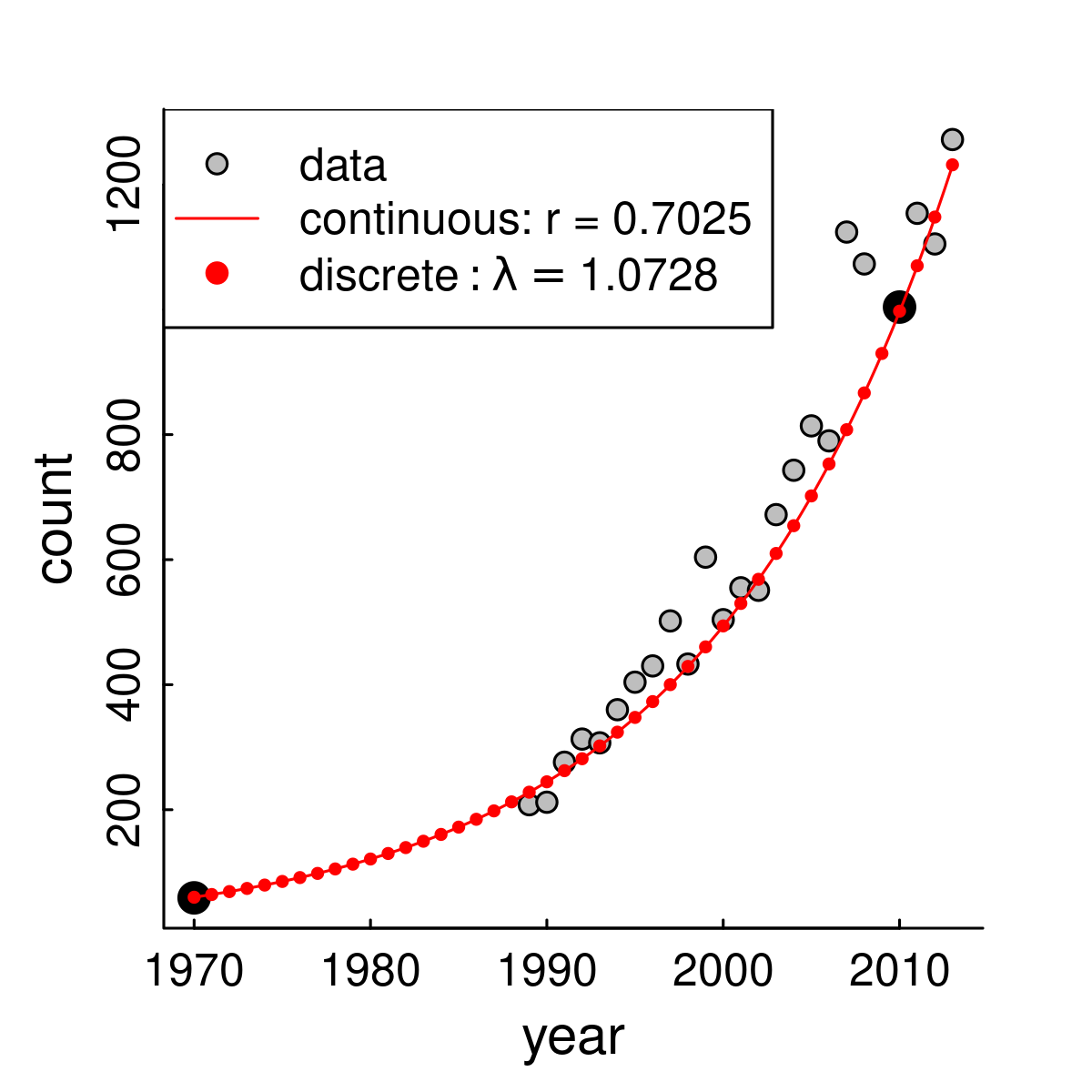] -- .pull-right[ ## Because ... ***randomness!(?)*** *What are some potential sources of "randomness" in the sea otter population process?* ] --- ## If the exponential model is so tidy ... why isn't it *perfect*? .pull-left-50[ ] .pull-right[ ## Because ... ***randomness!(?)*** *What are some potential sources of "randomness" in the sea otter population process?* >- Environment good / bad affecting all animals ... >- Randomness in birth-death affecting individual animals ... >- Unexpected immigration / emigration ... >- Observation error ... ] --- ## Brief Intro to Random Variables .pull-left.large[ Easiest problem in boring arithmetic: `$$\huge 1 + 1 = 2$$` ] .pull-right.large[ Easiest problem in random arithmetic: <br> <br> <center> <img src='images/coinflip.jpg' width='20%'/> `\(\huge +\)` <img src='images/coinflip.jpg' width='20%'/> `\(\huge = ?\)` </center> ] --- ## One coin flip is Random .large[Random variables have *possible events* associated with *probabilities*. ] event | numeric | probability :-----:|----|----- <img src='images/T.png' width='20%'/> | `\(\Large 0\)` | `\(\Large 1/2\)` <img src='images/H.png' width='20%'/> | `\(\Large 1\)` | `\(\Large 1/2\)` --- ## Two coin flips is also Random Random variables have *possible events* associated with *probabilities*. event | numeric | probability :-----:|----|----- <img src='images/T.png' width='10%'/><img src='images/T.png' width='10%'/> | `\(\Large 0\)` | `\(\Large 1/4\)` <img src='images/H.png' width='10%'/><img src='images/T.png' width='10%'/> `\(\,\,\Large \text{OR}\,\,\)` <img src='images/T.png' width='10%'/><img src='images/H.png' width='10%'/>| `\(\Large 1\)` | `\(\Large 1/2\)` <img src='images/H.png' width='10%'/><img src='images/H.png' width='10%'/> | `\(\Large 2\)` | `\(\Large 1/4\)` --- ## Random variables... ... are described by **Probability Distributions**. **Probability Distributions** have **names** and **parameters** that describe the distribution. <center> <img src="ExponentialGrowthWithStochasticity_files/figure-html/unnamed-chunk-3-1.png" width="80%" /> </center> One flip | = | `\(X \sim Bernoulli(p = 1/2)\)`. ---|---|--- **Two flips** | = | `\(X_1 + X_2 = Y \sim Binomial(p = 1/2, n=2)\)`. ** `\(n\)` flips** | = | `\(\sum_{i=1}^n X_i = Y \sim Binomial(p = 1/2, n=n)\)`. --- ## A bit about the binomial distribution .pull-left[ `\(X \sim Binomial(n, p)\)` describes the sum of `\(n\)` random events, each of which has probability `\(p\)`. ### Pop ecology example: If you have 20 sea otters ( `\(X_t = 20\)` ), each with a 90% probability of survival / year, how many next year? **Answer:** A random variable with distribution: `\(X_{t+1} \sim Binomial(n = 20, p = 0.9)\)` ] .pull-right[ <img src="ExponentialGrowthWithStochasticity_files/figure-html/unnamed-chunk-4-1.png" width="100%" /> ] --- ## Key questions about a random variable: `$$X_{t+1} \sim Binomial(n = X_t,\,\, p = p_{surv})$$` .pull-left[ ### Q1. How many would you *expect* to survive? `$$E(X) = \mu_X = np = 0.9 \times 20 = 18$$` This value is the **Expectation** of the distribution: `\(E(X)\)` or `\(\mu(X)\)`. It would be the *mean* value if you could repeat the experiment an infinite amount of times. ] .pull-right[ ### Q2. How much *variability* is there in this process? `$$SD(X) = \sigma_x = \sqrt{n\,p(1-p)} = 1.34$$` The **standard deviation** of a random variable: `\(SD(X)\)` or `\(\sigma_x\)` quantifies how concentrated the distribution is around the *mean*. *Approximately* 95% of the probability is within 2 standard deviations. ] --- ## Continuous random variables There are a bunch. The most famous is the **Normal** or **Gaussian** distribution: `$$X \sim {\cal N}(\mu, \sigma)$$` It has two parameters: `\(\mu\)` and `\(\sigma\)` with are - unsurprisingly - the *mean* (expectation) and *standard deviation* (spread) of the variable. .pull-left[ <img src="ExponentialGrowthWithStochasticity_files/figure-html/unnamed-chunk-5-1.png" width="100%" /> ] .pull-right[ <img src="ExponentialGrowthWithStochasticity_files/figure-html/unnamed-chunk-6-1.png" width="100%" /> ] --- ## Once upon a time in Germany ....  --- ## Some probability distributions We use these to **model** random processes: | name | notation | possible values | models | mean | standard deviation | |----|----|---|---|---|---| | Normal | `\({\cal N}(\mu, \sigma)\)` | `\((-\infty, \infty)\)` | bell-shaped | `\(\mu\)` | `\(\sigma\)` | | Exponential | `\(Exp( \lambda)\)` | `\([0,\infty)\)` | random events | `\({1\over\lambda}\)` | `\({1 \over \lambda}\)` | | Poisson | `\(Poisson(\lambda)\)` | `\([0,\infty)\)` | positive count data (e.g. births)| `\(\lambda\)` | `\(\sqrt{\lambda}\)` | | Bernoulli | `\(Bernoulli(p)\)` | `\([0,1)\)` | binary outcomes (e.g. deaths)| `\(p\)` | `\(\sqrt{p(1-p)}\)` | | Binomial | `\(Binomial(n, p)\)` | `\([0,n)\)` | many binary outcomes | `\(np\)` | `\(\sqrt{n p(1-p)}\)` | --- ## Demographic Stochasticity .large[ - ***Stochasticity*** means: **Randomness** in **time**. - ***Demography*** is the **Science of Population Dynamics**. Often it refers specifically to **births** and **deaths** (and **movements** ... but we're still looking at closed population). - Individually, *all* demographic processes are stochastic. An individual has some *probability* of dying at any moment. An individual has some *probability* of reproducting at a given time. Q: How important is *individual* randomness for a *population* process? More specific Q: **What is the probability of extinction?** ] --- class: inverse ## Human Experiment with Life and Death .pull-left-60.large[ - 15 students - Flip a survival coin. - If you die (**TAILS**) sit down, if you live (**HEADS**) stay standing - Flip a reproduction coin. - If you reproduce (**HEADS**) call on another student to stand ] .pull-right-40[] --- ## What do we predict from this experiment? Starting with `\(N_t\)`: expected number of survivors (S): `$$E(S) = p_s N_t$$` Expected number of new individuals (babies - B): `$$E(B) = p_b E(S)$$` New population equals survivals + new babies: `$$E(N_{t+1}) = E(S) + E(B) = p_s N_t + p_b\,p_s N_t = p_s(1 + p_b) N_t$$` So (in our coin flip example) `$$\widehat{\lambda} = p_s (1+p_b) = 0.75$$`. .center[**What does that mean for population growth!?**] --- ## Cranking this experiment very many times. https://egurarie.shinyapps.io/StochasticGrowth/ .center[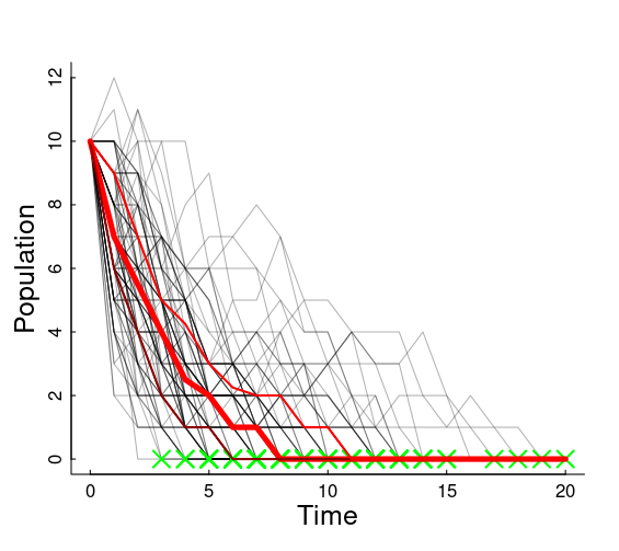] --- ## Some predictions for a similar continuous model .pull-left[ Assume birth rate `\(b\)` and death rate `\(d\)`, and growth rate `\(r = b-d\)`. The mean of the process is also exponential growth `$$E(N_t) = N_0 e^{r t}$$` If birth rate = death rate: `$$SD(N_t) \approx \sqrt{2 N_0 b t}$$` Note, increases as square root of time. There's a somewhat more complex formula for births `\(\neq\)` deaths. ] .pull-right[ More importantly: `$$\begin{equation} P(extinction) = \begin{cases} \text{if}\,\,b > d;& (d/b)^{N_0}\\ \text{if} \,\, d > b;& 1 \end{cases} \end{equation}$$` Note that even when birth rate = death rate, `\(P(extinction) = 1\)`, i.e. eventual extinction is certain. This is very similar to the eventual probability of fixation for genetic drift. Also, probability of extinction is lower for smaller `\(N_0\)`. ] --- ## Environmental Stochasticity... .pull-left-40[ Some random aspect of the environment that influences .blue.large[***r***] (whether via .green[births] or .red[deaths] or **both**) for the **entire population**.: `$$R \sim Dist(\mu_r, \sigma_r)$$` - `\(\mu_r\)` is the *mean growth rate* - `\(\sigma_r\)` is the *variability on the growth rate* ] -- .pull-right-60[ > .darkred[**Can you think of some examples, e.g. for sea otters?**] ] --- ## Environmental Stochasticity... .pull-left-40[ Some random aspect of the environment that influences .blue.large[***r***] (whether via .green[births] or .red[deaths] or **both**) for the **entire population**.: `$$R \sim Dist(\mu_r, \sigma_r)$$` - `\(\mu_r\)` is the *mean growth rate* - `\(\sigma_r\)` is the *variability on the growth rate* ] .pull-right-60[ > .darkred[**Can you think of some examples, e.g. for sea otters?**] 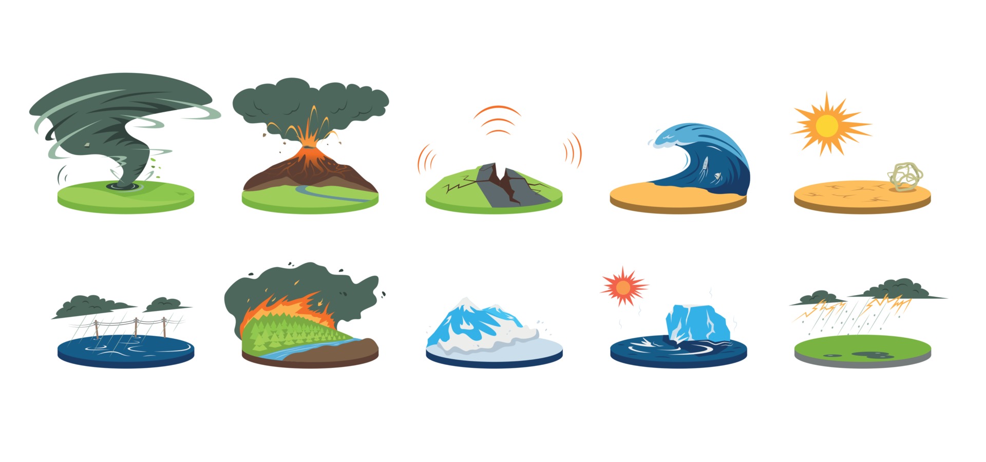 ] --- class: inverse ## Human Experiment .pull-left-60.large[ The **professor** IS the **environment**! 1. `$$\large N_0 = 16$$` 2. If the environment flips **Heads**, the population doubles. 3. If the environment flips **Tails**, the population halves. ] .pull-right-40[] --- ## Environmental Stochasticity: Analysis .pull-left-40[ This model can be written: `$$N_{t+1} = N_t \, 2^{R}$$` Where `\(R\)` is a random variable: value | prob. ---|--- -1 | 1/2 +1 | 1/2 ] .pull-right[ `$$E(R) = \mu_r = 0$$` So population should not grow, on average. `$$E(N(r)) = N_0 e^{\mu_r t} = N_0$$` And: `$$SD(R) = \sigma_R = 1$$` ] -- >- Are you doomed to extinction? >- Does this remind you of another process from earlier in class? .center[Experiment here: https://egurarie.shinyapps.io/StochasticGrowth] --- ## A stochastic population is a random variable! .pull-left-40[ `$$N(t) \sim Dist(\mu_N(t), \sigma_N(t))$$` The mean / expectation is the same as for the exponential growth function, but with the mean growth rate substituted: `$$\mu_N(t)= N_0 e^{\mu_r t}$$` But the standard deviation of the function increases with time! `$$\sigma^2_{N}(t) \approx N_0\,e^{\mu_r t} \sqrt{e^{\sigma_r^2t} - 1}$$` ] .pull-right-60[ Sea otter example, with `\(\mu_r = 0.07\)` and `\(\sigma_r = 0.07\)`: 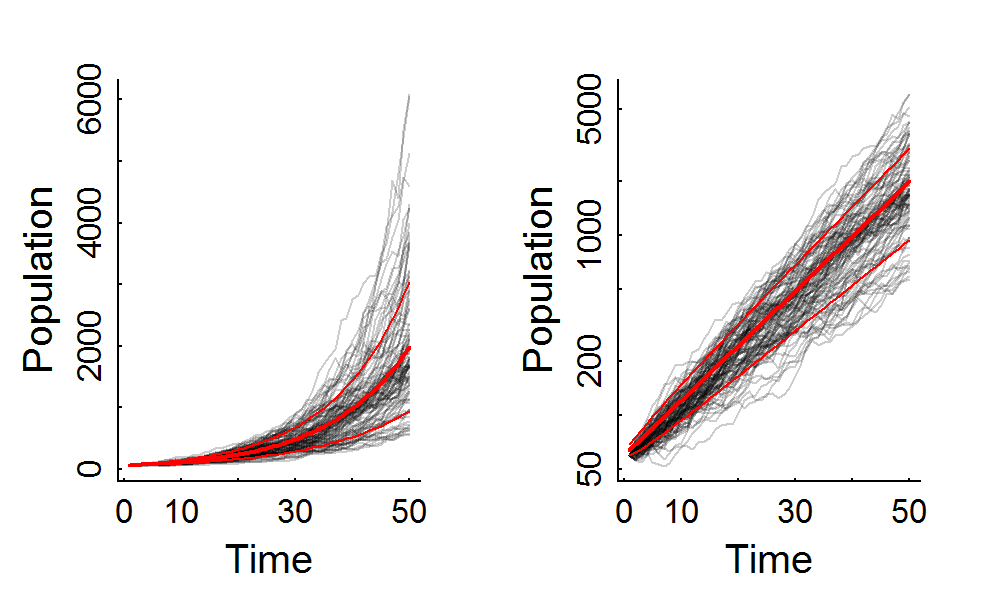<!-- --> Grey lines are simulations. Red lines are `\(\mu_N(t) \pm \sigma_N(t)\)` ] --- .large.pull-left-60[ ## If things are TOO random that spells trouble! According to theory, if: .darkred[$$\sigma_r > 2\mu_r$$] extinction is nearly certain - even if `\(\mu_r\)` is positive and on average there is growth. > .center[Experiment here: https://egurarie.shinyapps.io/StochasticGrowth] ] .pull-right-40[ ] --- class: inverse .pull-left-60.large[ ## Key Takeaways 1. Nature is a combination of **very complex** and **truly random**. So we have to get comfortable with randomness 1. **Demographic stochasticity** refers to **individual randomness**, and particularly effects **small populations**. 2. **Environmental stochasticity** affects **everyone similarly**, **big** or **small** populations, and too much randomness bodes ILL. ] .pull-right-40[ . ]