Exponential Growth: Part I

class: center, top, title-slide

.title[
# <strong>Exponential Growth: Part I</strong>
]
.subtitle[
## <a href="https://eligurarie.github.io/EFB370/">EFB 370: Population Ecology</a>
]
.author[
### <strong>Dr. Elie Gurarie</strong>
]
.date[
### <strong>February 12, 2024</strong>
]

---

.pull-left[

## Goals 
### (concepts / buzzwords / jargon)

- The Population Equation 
- Closed vs. Open Population 
- Unconstrained (density independent) Growth
- Geometric Growth = Exponential Growth
- Discrete Time vs. Continuous Time Models
- Difference Equations vs. Differential Equations
- Population growth parameters: 
  - continuous / discrete / per capita / per unit time
- Amazing properties of exponential and log.
]

.pull-right[

## *Suggested* reading

- Gotelli: Chapter 1 (first half)
- Neal: Chapter 4
]

---
class:Large

## Meet ... *Enhydra lutris*

The largest ...

.center[**Mustelid**]

The smallest ...

.center[**Marine mammal**]

By far the furriest! Guess how may hairs / sq. inch ?

(*Hint, humans are born with  ~100,000 TOTAL.* )

.center[**1,000,000** (ish!)]

---

## Sea otters: Range

.pull-left-60[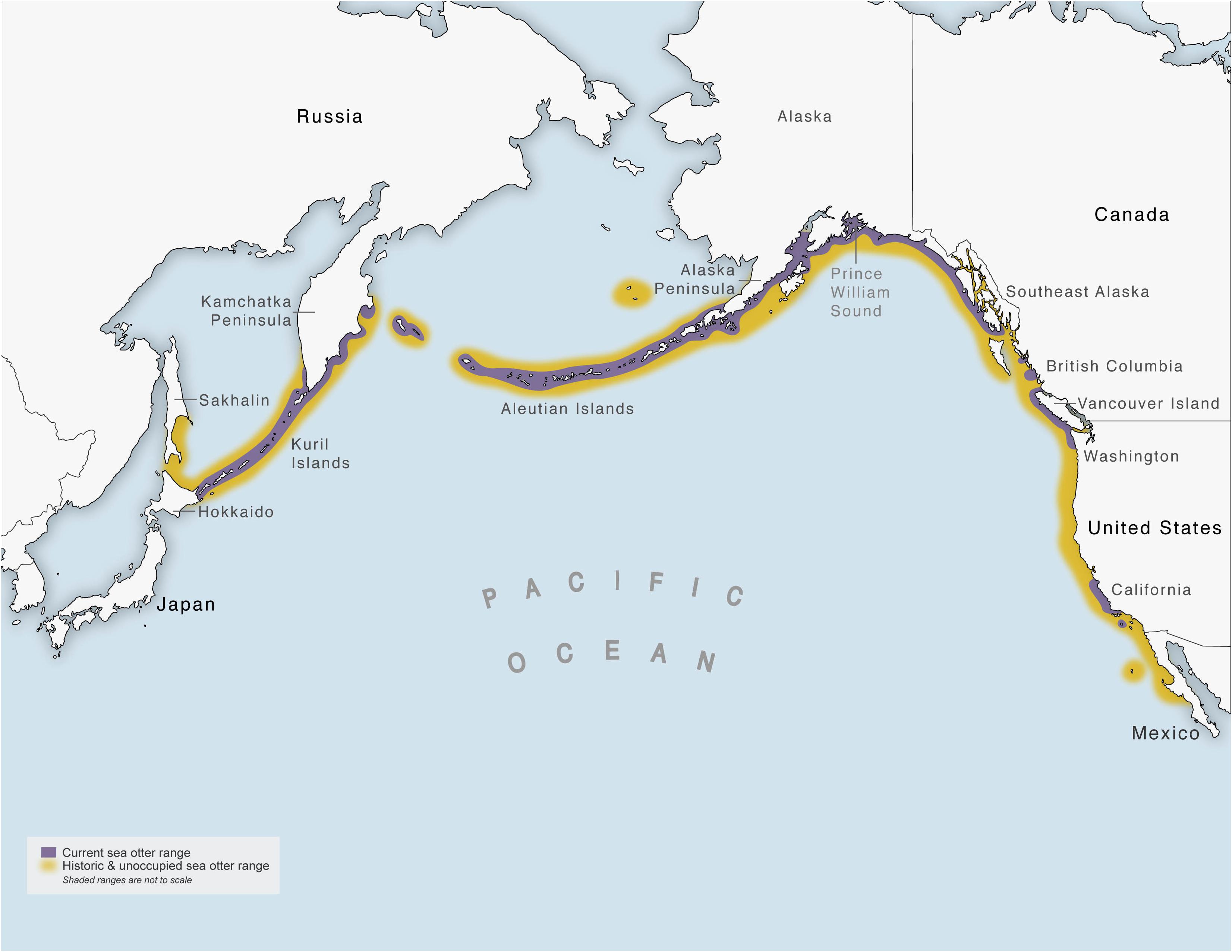![](images/range.jpg)]
.pull-right-40.Large[*Littorally* the entire North Pacific]

---

## Sea otters: Keystone Species

![](images/seaotter_foodweb.jpg)

(Estes et al. 1974)

---

.pull-left-50[

## Sea otters: Furriness > Cuteness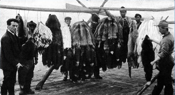

![](images/furtrade.jpg)
]

.pull-right-30[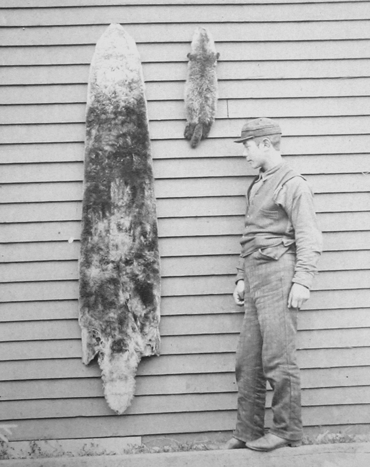

![](images/furs.jpg)
]
.pull-left[
- Fur trade (Russian -> British -> American) leads to near **extirpation** across the entire range.
- **> 300,000 in 1740 ... < 2,000 in 1900**.  
- Displacement and indenturing of Indigeneous fishermen (esp. Aleut)
]
.pull-right[
> .footnotesize[*... the rush for the otters’ “soft gold” was a predictable boom and bust ... a cautionary example of unsustainable resource use, and a socioeconomic driver of Western — mainly American — involvement in the Pacific region,*  (Loshbaugh 2021)]

]

---

.pull-left[
## Sea otters: Not totemic

.box-grey[
... a sea otter hunter who was “lazy, spiteful, malicious or disregarded the teaching of the elders” would find his prey “cavorting around his baidarka ... teas[ing] and splash[ing] him with water.”  *(Innokentiy Venianimov, 1840)*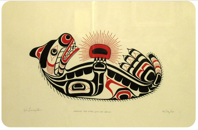
]

![](images/seaotter_JohnLivingston.png)
.center[*art by John Livingston*]

]

.pull-right[
### ... but culturally significant
 
<iframe src="https://www.youtube.com/embed/ZyYH4KBHKU4?controls=0" width = "400" height = "240">
</iframe>

.small[See: https://www.youtube.com/watch?v=ZyYH4KBHKU4]

.scriptsize[

.pull-left[
| culture | name |
|---|---|
| [Ainu](https://en.wikipedia.org/wiki/Ainu_people) | Esaman |
| [Koryak](https://en.wikipedia.org/wiki/Koryaks) | Kolakha |
| [Aleut](https://en.wikipedia.org/wiki/Aleut) | Chngatux |
| [Alutiiq](https://en.wikipedia.org/wiki/Alutiiq) | Arhnaq |
]

.pull-right[
| culture | name |
|---|---|
| [Tlingit](https://en.wikipedia.org/wiki/Tlingit) | Yáxwchʼ |
| [Haida](https://en.wikipedia.org/wiki/Haida) | Ku |
| [Nuu chah nulth](https://en.wikipedia.org/wiki/Nuu-chah-nulth) | Кwak̕aƛ |
| [Siletz](https://en.wikipedia.org/wiki/Siletz) | Elakha |
]
]
]

---

## Sea otter reintroduction: Pacific NW

Remnant populations from Aleutian Islands ... released in OR, WA, BC and SE-AK  1969 – 1972.

.center[
<img src="images/introduction.jpg" alt="Reintroduction trade" height="300"/>
<img src="images/introduction2.jpg" alt="Reintroduction trade" height="300"/>
]

---

## Sea otter reintroduction: Washington State ...

.pull-left[![](images/wa_range.png)]
.pull-right[
.pull-left[1970: **59 otters**]
.flush-right[2010's: **over 1000**]

![](plots/WA_popgrowth.png)
]

---

## Sea otter reintroduction: Washington State ...

.pull-left[![](images/wa_range.png)]
.pull-right[
.pull-left[1970: **59 otters**]
.flush-right[2010's: **over 1000**]

![](plots/WA_popgrowth2.png)

]

.center.Large[***Success!***]

---

## Population ecology is all about ...

`$$\huge N$$`

but where?  when?

## Here! Now! ..

`$$\huge N_t$$`

but how many were there?

---

## That many, then `$\Delta t$` ago!

`$$\Large N_t = N_{t - \Delta t} + \Delta N$$`

slight rearrangement:

`$$\Large N_{t+1} = N_t + \Delta N$$`

For now, `$\Delta t = 1$`, i.e. it's the discrete unit that we measure population change.  VERY TYPICALLY - whether because of biology or field seasons:  `$$\Delta t = 1\,\, \textrm{year}$$`.

---

## How does population change?

`$$\Large N_{t+1} = N_t + (B - D) + (I - E)$$`

### **B**irth
### **D**eath
### **I**mmigration
### **E**migration

---
  
## Assumption 1: no one's getting on or off the bus

`$$\Large N_{t+1} = N_t + B - D$$`

### **B**irth
### **D**eath

### ~~.red[**I**mmigration]~~
### ~~.red[**E**migration]~~

.center[This is a .darkblue[**closed**] (vs. **open**) .darkblue[**population**] ...]

---

## Assumption 2: the important one

The number of *Births* and *Deaths* is proportional to *N*.

`$$\Large N_{t+1} = N_t + bN_t - dN_t$$`
*b* and *d* are number of births and deaths *per individual*.   What does that mean?

.pull-left[
.box-yellow[**Births**

- Every female gives birth to the same number of offspring?

- Every female has the same *probability* of giving birth to a single offspring?

- Every female has the same *probability* of giving birth to the same *distribution* of offspring?]
]

.pull-right[
.box-green[
**Deaths**

- A fixed proportion of all individuals dies?

- Every individual has the same *probability* of dying?

- the *distribution* of *probabilities* of dying is constant? 
]]

.center.large[**These are all subtly & importantly different!**]
---

## Some math ....

Define `$$r_0 = b - d$$`

`$r_0$`: **discrete growth factor**,

`$$N_{t+1} = N_t + r_0 N_t$$`
`$$N_{t+1} = (1 + r_0) N_t$$`

`$$N_{t+1} = \lambda N_t$$`

`$\lambda$` is .blue[**rate of growth (or decrease)**]

- If `$d > b$`, `$\lambda < 1$`.  
- If `$b > d$`, `$\lambda > 1$`.

---
 
## Cranking this forward

`$$N_{t+1} = \lambda(N_t)$$`
`$$N_{t+2} = \lambda(N_{t+1}) = \lambda^2 N_t$$`
`$$N_{t+3} = \lambda^3 N_t$$`

Solution:

`$$\large N_{t+y} = \lambda^y N_t$$`
or

`$$\huge N_t = \lambda^t N_0$$`

.center[***Geometric*** (same as ***Exponential***) growth.]

---

## Some examples

![](ExponentialGrowth_PartI_files/figure-html/LambdaExamples2-1.png)

---

## How fast is exponential/geometric growth?

.pull-left-60[
![](images/chess.jpg)

Legend says the inventor of chess (in India) so delighted the raja, he was offered anything he wanted.

Inventor said, not much.  One grain of rice on one square, 2 on the next, 4 on the next and so on till the board is filled. 
]
 
--

.pull-right-40[
![](images/chessrice.jpg)

Not only is there not enough rice in India to fill such a chessboard, **there are not enough atoms on earth**.  
]
---

## Note what the log-scale does

![](ExponentialGrowth_PartI_files/figure-html/LambdaExamples-1.png)

---

## Estimating some rates ... discrete

.pull-left-30[![](images/seaotter_cute.jpg)]

.pull-right-70[

The amazing thing is, if you have an equation "solved", you only need 2 points on the curve to compute.

Let's use the discrete equation:

`$$N_{t+y} = \lambda^y N_t$$`
`$$1000 = 60 \times \lambda^{40}$$`
`$$16.7 = \lambda^{40}$$`
`$$2.81 = 40 \times \log (\lambda)$$`
`$$0.07025 = \log (\lambda)$$`
`$$\lambda = \exp(0.07025) = 1.0728$$`

i.e. population increase about `$$7.28\%/year$$`. 
]

---

## Washington sea otter fit to data (7.025% discrete growth)

.pull-left-70[
![](images/SeaOttersFitted.png)
![](ExponentialGrowth_PartI_files/figure-html/unnamed-chunk-4-1.png)
]

.pull-right-30[
### This is an EXCELLENT fit

but why isn't it *perfect*?

.darkgreen[What are some potential sources of **variation**?]
]

---
## Discrete Model to Continuous Model

.pull-left[

Let's do some trickery, starting with:
`$$N_{t+1} = (1 + r_0) \, N_t$$`
`$$N_{t+1} - N_t = r_0 N_t$$`
`$$N_{t+\Delta t} - N_t = r_{\Delta t} N_t$$`

`$$\lim_{\Delta t \to 0} {\Delta N \over \Delta t} =  \lim_{\Delta t \to 0}  {r_{\Delta t} \over \Delta t} N$$`
]

.pull-right[

Magically define: 
`$${r_\Delta \over \Delta t} = r$$` and rewrite `$\Delta$` as `$d$`:

.blue[$$\large {dN \over dt} = r N$$]

> .darkblue.large[This is a ***differential*** (vs. difference) equation]

]

---

.large.green[**Solve this:**
 `$$\large {dN \over dt} = r N$$`]
 
 where: `$$N(t = 0) = N_0$$`

.pull-left[
.small[Integration is fun!  (*but you don't need to know how to do this*)]

`$$\begin{align}
    {1\over N} dN &= r dt \\
    \int_{t' = t_0}^t {1 \over N(t)} dN &= \int_{t' = t_0}^t r dt  \\
    \log(N) &= rt + C_0 \\
    N &= e^{rt + C_0} \\
\end{align}$$`

]

.pull-right[
.large.red[**Solution:**
`$$\large N(t) = N_0 e^{rt}$$`]

> **Incredibly Interesting And Important Fact:**

>The exponential function is the ONLY function whose derivative is proportional to itself.

]

---

## Some examples

![](ExponentialGrowth_PartI_files/figure-html/ContinuousGrowth-1.png)

---

.pull-left[
## Note crazy fast growth

![](ExponentialGrowth_PartI_files/figure-html/ContinuousGrowth_v2-1.png)
]

.pull-right[
## and how straight on a log-scale

![](ExponentialGrowth_PartI_files/figure-html/ContinuousGrowth_v3-1.png)
]

---

## Discrete vs. Continuous Modeling

.pull-left[

**Difference equations**
`$$N_{t+\Delta t}  - N_t = \lambda_{\Delta t} N_t$$`

think of *absolute change*

**Pros:**

- Reflects (often) biological reproduction patterns, practical sampling schedule (esp. annual)
- Intuitive

**Cons:**

- Depends on discretization timescale
- Surprisingly difficult to analyze
]

.pull-right[

**Differential equations**
`$${dN \over dt} = r N$$`

think of *rates* (change/time).

**Pros**

- Easier "elegant" mathematical analysis
- Scales nicely

**Cons**

- Unbiological 
- Unintuitive
]

---

## Estimating some rates ... continuous

.pull-left-30[![](images/seaotter_cute.jpg)]

.pull-right-70[

Let's use the continuous equation:

`$$\begin{align} 1000 &= 60 \times e^{40\,r}\\
16.7 &= e^{40 \, r}\\
2.81 &= 40 \times r\\
r &= 0.07025
\end{align}$$`
.large[*Intrinsic growth rate* = 0.07025.]
]

---

## Washington sea otter fit to data
.pull-left[
![](ExponentialGrowth_PartI_files/figure-html/WAfit2-1.png)
]

.pull-right[
Note: dots for **discrete**, lines for **continuous** ...

.green[*but really there is NO difference in the two curves*]
]

---

## Estimating some rates ... discrete

.pull-left-30[![](images/seaotter_cute.jpg)]

.pull-right-70[

The amazing thing is, if you have an equation "solved", you only need 2 points on the curve to compute.

Let's use the discrete equation:

`$$N_{t+y} = \lambda^y N_t$$`
`$$1000 = 60 \times \lambda^{40}$$`
`$$16.7 = \lambda^{40}$$`
`$$2.81 = 40 \times \log (\lambda)$$`
`$$0.07025 = \log (\lambda)$$`
`$$\lambda = \exp(0.07025) = 1.0728$$`

i.e. population increase about `$$7.28\%/year$$`. 
]

---

## How long does it take for a population to double?

.center.large[ 
solve for doubling time `$t_d$` 
]

.pull-left.large[
**Continuous:**

`$$2N = N e^{rt_d}$$`
`$$\log(2) = rt_d$$`
`$$t_d = \log(2)/r$$`
]

.pull-right.large[**Discrete:**

`$$2N = N \lambda^{t_d}$$`
`$$\log(2) = \log(\lambda) t_d$$`
`$$t_d = \log(2)/\log(\lambda)$$`
]

.center.large[

> Sea otter population doubles in ~10 years.

]

---

## Some sea otter references

.pull-left[

- J. A. Estes, J. F. Palmisano. 1974. Sea otters: Their role in structuring nearshore communities. Science 185, 1058–1060. ([link](https://www.science.org/doi/10.1126/science.185.4156.1058))

- Loshbaugh S. 2021. Sea Otters and the Maritime Fur Trade. In: Davis R.W., Pagano A.M. (eds) *Ethology and Behavioral Ecology of Sea Otters and Polar Bears. Ethology and Behavioral Ecology of Marine Mammals.* ([link](https://link.springer.com/chapter/10.1007/978-3-030-66796-2_10))

- Gilkinson, A.K., Pearson, H.C., Weltz, F. and Davis, R.W., 2007. Photo‐identification of sea otters using nose scars. *The Journal of Wildlife Management*, 71(6), pp.2045-2051.  ([link](https://doi.org/10.2193/2006-410))

-  Veltre, D.W. *Unangax̂: Coastal People of Far Southwestern Alaska*. ([link](https://www.apiai.org/departments/cultural-heritage-department/culture-history/history/))

]

.pull-right[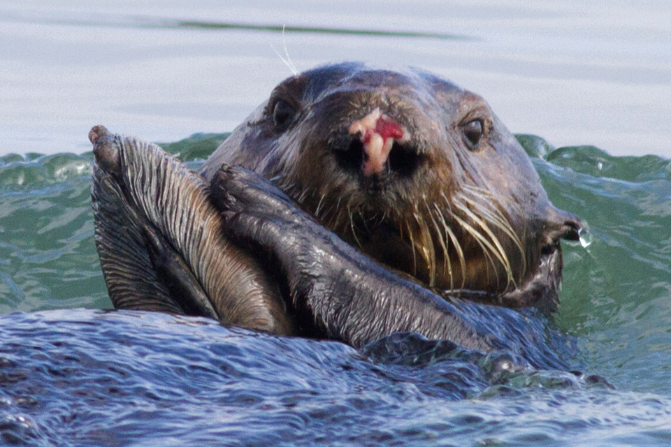
![](images/otter_nosescar.webp)

If you want to disabuse yourself of "sea otters are cute" - read about why the females have nose scars. 
]