class: left, top, inverse, title-slide .title[ # <strong>Life History Tables</strong> ] .subtitle[ ## <a href="https://eligurarie.github.io/EFB370/">EFB 370: Population Ecology</a> ] .author[ ### .white[<strong>Drs. Elie Gurarie</strong> and <strong>Nate Wehr</strong>] ] .date[ ### .white[March 6, 2023] ] --- ## Learning Life History Tables .pull-left-70[ 1. **Survival** and **Fecundity** vary with age / class / stage 2. **Life history tables** organize that variability: - age distribution `\(S(x)\)` - survival schedule `\(l(x)\)` - birth schedule `\(b(x)\)` 3. With those schedules we can compute: - **Growth rate** `\(r\)` - **Generation time** `\(G\)` - **Stable age distribution** `\(N^*\)` - **Reproductive value** `\(v_x\)` *(But the calculations are fussy!)* 4. Different schedules point to different **life history strategies** ] .pull-right-30[  ] --- ## Life Table analysis .pull-left-60[ A "schedule" of all births and deaths in our population - .darkblue[**Fecundity schedule:**] *how many* offspring are born by **age** - .darkred[**Survivorship schedule:**] *with what probability* individuals by **age** With those (& some tedious calculations) you can compute: - **Life expectancy** - Population **growth rate** `\(\lambda\)` .green[important note: ALL of these models are *discrete exponential* growth models] - **Age structure:** Are there lots of: young individuals? Old individuals? Reproductive age individuals? - **Survivorship patterns** .green[Does most mortality occur in the very young? The very old? Or equally across all ages?] ] .pull-right-40[  ### Life history ***strategy*** Often - beyond a description - the real question is what influences or explains these parameters? - evolutionary - environmental - density dependent - human impacts ] --- ## Life Tables - some "encouragement" <img src='images/gotelliencouragement.png' width='100%'/> ### Two main pieces: - **Fecundity schedules:** Number of births per age class - i.e. reproductive contributon of females - **Survivorship schedules:** Number of deaths or probability of death per age class. --- ## Remember *Monoceros academicus* . | Larva | Sophomore | Emeritus | --- |:----------:|:------:|:---:| . | <img src='images/unicornlarva.webp' height='150px'/> | <img src='images/unicornstudent.jpg' height='150px'/> | <img src='images/oldunicorn.webp' height='150px%'/> | <font size = 5> Survival | <font size = 5> 0.5 |<font size = 5>1 | <font size = 5>0 | <font size = 5> Fecundity |<font size = 5> 0 | <font size = 5>1.5 | <font size = 5>0.5 | |||| > - **Survival** is a **probability** (unitless) > > - **Fecundity** is an **expected number** of offspring (n. ind.). </center> --- .pull-left-40[ ## Experiment: results Stage | Survival | Fecundity ----------|------|--- 1. larvae | 0.5 | 0 2. sophomore | 1 | 1 3. emeritus | 0 | .5 See numerical experiment: https://egurarie.shinyapps.io/AgeStructuredGrowth/ ] .pull-right-60[ <img src="PopulationStructure_PartII_files/figure-html/runPop1-1.png" width="100%" /> >- Eventually obtains a 2:1:1 stable age distribution >- Overall growth ($\lambda$)= 1 ] --- ## Survivorship schedules .pull-left-60[  ] .pull-right-40[ - **TYPE I:** high survivorship for juveniles; most mortality late in life - **TYPE II:** survivorship (or mortality) is relatively constant throughout life - **TYPE III:** low survivorship for juveniles; survivorship high once older ages are reached ] --- ## The pieces (columns): <font color = "green"> **Age class** `\((x)\)` </font>| <font color = "green"> **Number at Start** `\((S_x)\)` </font> | Cum. Prob. of survival `\((l_x = S_x/S_1)\)` | <font color = "green"> **births/ind** `\((b_x)\)` </font> | Surv. prob `\((g_x = l_x - l_{x+1})\)` | Rep. rate: `\((l\times b)\)` | `\(g = lbx\)` ---|:---:|:---:|:---:|:---:|:---:|:--:| 1. larva | **16** | | **0** | | | 2. sophomore | **8** | | **1.5** | | | 3. emeritus | **8** | | **.5** | | | 4. beyond | **0** | 0 | -- | -- | -- | -- **totals:** | `\(\Sigma S_i = 32\)` | `\(\Sigma D_i = S_1 = 16\)` | | | `\(R_0 = \sum lb\)` | `\(G = {\sum(lbx) \over \sum(lb)}\)` Goals: 1. Fill out table 2. compute reproductive rate: `\(R_0\)` - mean number of offspring / female 3. compute eneration time: `\(G\)` - mean age of mother --- ## The pieces (columns): <font color = "green"> **Age class** `\((x)\)` </font>| <font color = "green"> **Number at Start** `\((S_x)\)` </font> | Cum. Prob. of survival `\((l_x = S_x/S_1)\)` | <font color = "green"> **births/ind** `\((b_x)\)` </font> | Surv. prob `\((g_x = l_x - l_{x+1})\)` | Rep. rate: `\((l\times b)\)` | `\(g = lbx\)` ---|:---:|:---:|:---:|:---:|:---:|:--:| 1. larva | **16** | 1.0 | 0 | 0.5 | 0 | 0 2. sophomore | **8** | 0.5 | 1.5 | 1 | 0.75 | 1.5 3. emeritus | **8** | 0.5 | .5 | 0 | 0.25 | .75 4. beyond | **0** | 0 | -- | -- | -- | -- **totals:** | `\(\Sigma S_i = 32\)` | `\(\Sigma D_i = S_1 = 16\)` | | | `\(R_0 = 1\)` | `\(G = 2.25\)` --- ## *Monoceros academicus*: Type I .pull-left[ <img src="PopulationStructure_PartII_files/figure-html/MonocerusTypeI-1.png" width="100%" /> ] .pull-right[ - **TYPE I:** high survivorship for juveniles; most mortality late in life. Investment in young and survival. Typical of long-lived species. Stage | Survival | Fecundity ----------|------|--- 1. larvae | 0.5 | 0 2. sophomore | 1 | 1.5 3. emeritus | 0 | .5 ] --- .pull-left-70[ ## Pink Salmon (*Onchorrhynchus gorbusha*) .pull-left[] .pull-right[] ] .pull-right-30[ ### Strict 2-year life cycle Year 0: - Spawn in late-summer - Hatch in winter - Emerge in spring Year 1: - Ocean phase Year 2. - Enter freshwater late spring - Spawn - Die ] --- ## Pink Salmon (*Onchorrhynchus gorbusha*): Type III .pull-left[ <img src="PopulationStructure_PartII_files/figure-html/OnchorhynchusTypeII-1.png" width="100%" /> ] .pull-right[ - **TYPE III:** low survivorship for juveniles; survivorship high once older ages are reached. Basically - produce a whole boatload of offspring and hope for the best. Typically short-lived species. Stage | Survival | Fecundity ----------|-------|--- 1. smolt | 0.05 | 0 2. ocean | 0.9 | 0 3. return | 0 | 21 ] --- ## You can use life-history tables to compute: .pull-left-60[ **Stable Age Distributions:** `$$c(x) = {e^{-rx} l(x) \over \sum_{x = 0}^k e^{-rx} l(x)}$$` **Reproductive value** (.darkgreen[Number of offspring YET to be born.]) `$$v(x) = {e^{rx}\over l(x)} \sum_{y = x+1}^k e^{-ry} \, l(y)b(y)$$` **Growth rate** approximately: `\(r \approx \log(R_0)/G\)`, or exactly solve this: `$$1 = \sum_{x=1}^n e^{-rx} l(x) b(x)$$` for `\(r\)`. ] .pull-right-40[ 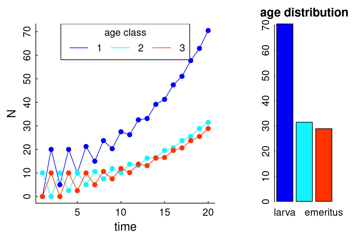 > Note how growth rate affects **stable age distribution**! ] --- ## Assumptions ... are the same as exponential growth: 1. Closed population 2. No genetic structure (or individual variability) 3. No time lags 4. Stationarity: - Exp. growth: `\(b\)` and `\(d\)` (birth and death rates) constant - Stage structured growth: `\(l(x)\)` and `\(b(x)\)` schedules are invariant in time. **The really interesting ecological questions ask what happens when conditions change** --- ## Ways of calculating ... 1. Through time: **Cohort analysis** - follow a cohort (or several cohorts) through time 2. Snapshot: **Age distribution** - almost always something weird turns up! 3. Mark-racapture, observational analysis of survival and reproduction If you have **N-1 variables** you can often infer the **missing one**! .pull-left[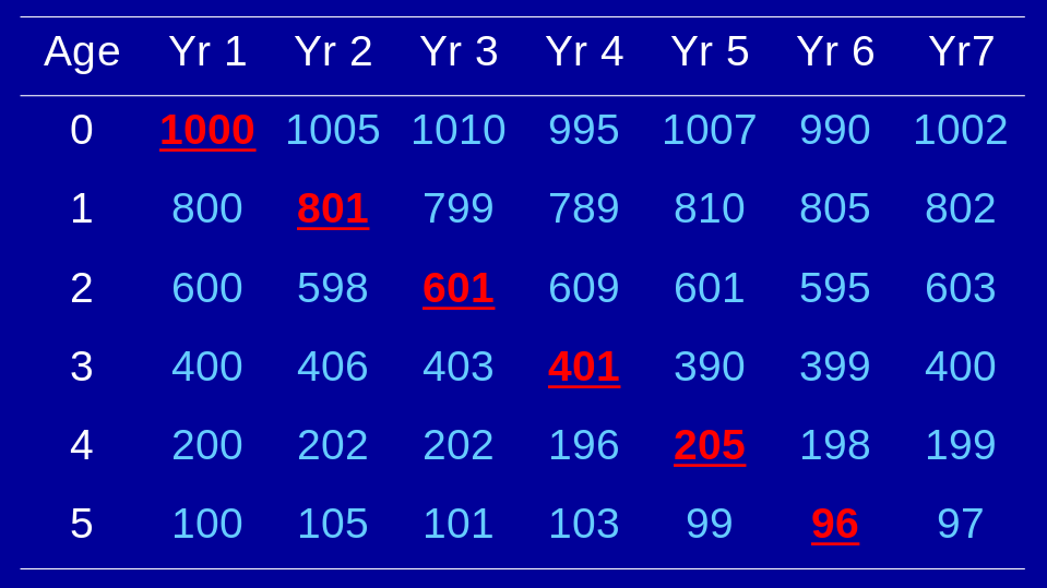] .pull-right[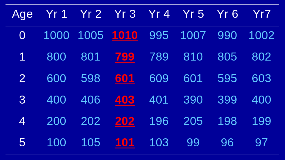] --- ## Fecundity Schedule .pull-left[ #### semelparous | monocarpic Reproduce ONCE (e.g. .blue[Pacific salmon / desert flower / annual plant]) Typical Schedule: .red[0-0-0-0-0-1000] ] .pull-right[ #### iteraoparous | polycarpic Reproduce many times (e.g. .blue[rabbit / elephant / human / oak]) Typical schedule: .red[0-10-10-10-10-10] ]  --- ## Estimating Life Histories: **Cohort Life Table** .large[Follow a cohort (or cohorts) through time. Track **survival**. Track **age at birth**.] .pull-left-40[ .large[ **Minus:** - Can take a really long time! **Plus:** - Population always decreasing! ]] .pull-right-60[  ] --- ## Estimating Life Histories: **Vertical Life Table** .large[Take a snapshot of the age distribution and build survival schedule] .pull-left-40[ .large[ **Strong assumptions:** - `\(r = 0\)` or `\(\lambda = 1\)` - processes (birth and survival schedules) are **stationary**, meaning .green[*parameters* don't change over time.] - Of course - you also need to know **birth schedule**. ] ] .pull-right-60[  ] --- ## Do these assumptions hold? US population pyramid - 2020 .pull-left-70.pull-right-70[ 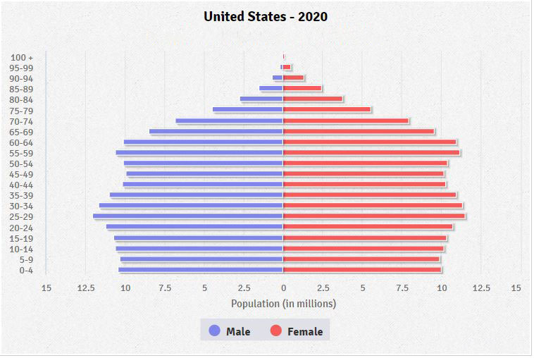 ]