class: left, top, title-slide .title[ # Interactions Part III: <strong>Functional Responses</strong> ] .subtitle[ ## <a href="https://eligurarie.github.io/EFB370/">EFB 370: Population Ecology</a> ] .author[ ### <strong>Dr. Elie Gurarie</strong> ] .date[ ### April 3, 2024 ] --- ## Isoclines ... Separate **phase space** into areas of increasing and decreasing **prey** or **predator** abundance. .pull-left[ <img src="Interactions_PartIII_FunctionalResponses_files/figure-html/unnamed-chunk-2-1.png" width="100%" /> ] .pull-right[ <img src="Interactions_PartIII_FunctionalResponses_files/figure-html/unnamed-chunk-3-1.png" width="100%" /> ] --- ## Lotka-Volterra If isoclines are perpendicular ... eternal oscillations. .center[ <img src='images/LVtrajectories.png' width='50%'/> ] --- ## Lotka-Volterra with Carrying Capacity If isoclines tilts ... damped oscillations .center[ <img src='timages/02_DDinPrey.png' width='80%'/> ] --- .center[## What if prey isocline is humped?] .pull-left[On the left **Allee effect** - too few prey = harder for population to grow.] .pull-right[On the right **Carrying capacity** - too many prey = density dependence kicking in] <br> .center[ <img src='timages/03_Parabola.png' width='65%'/> ] --- ## In the middle - stable oscillations .center[ <img src='timages/Got1_middle.png' width='60%'/> ] --- ## In the right - damped oscillations .center[ <img src='timages/Got2_right.png' width='65%'/> ] --- ## In the left - unstable oscillations .center[ <img src='timages/Got3_left.png' width='60%'/> ] --- ## Unintuitive result ... By increasing carrying capacity of prey ... you can send the system into an unstable state and INCREASE the probability of extinction. .center[ <img src='timages/Rosenzweig.png' width='75%'/> ] --- ## Rosenzweig's "enrichment paradox" .Large[ *“...increasing the supply of limiting nutrients or energy tends to destroy the steady state. Thus man must be very careful in attempting to enrich an ecosystem in order to increase its food yield. There is a real chance that such activity may result in decimation of the food species that are wanted in greater abundance.”* - Rosenzweig (1971) ] --- ## Nice theory you've got there .... .large[But is it real?] .center[ <img src='images/UnicellularPredation.jpg' width = '80%'/> ] .large.center[More experiments with *Didinium nausutum* vs. *Paramecium caudatum*.] --- ## High carrying capacity .center[<img src='timages/Luckinbill_HighC.png' width = '90%'/> .large[[Luckinbill 1973](https://doi.org/10.2307/1934194) recreates Gause experiments with a different food source.]] --- ## Low carrying capacity .center[<img src='timages/Luckinbill_LowC.png' width = '90%'/> .large[When the food source is limited ... more stable oscillations!]] --- ## Consistent with Enrichment Paradox ... .pull-left-40[ 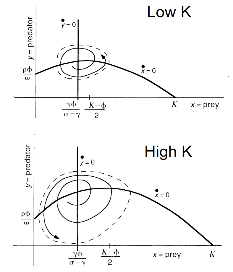 [Harrison (1995)](https://doi.org/10.2307/1941195) ] .pull-right[ ### HOWEVER, in natural systems... efforts to show this effect generally fail. (reviewed in [Roy and Chattopadhyay 2007](https://doi.org/10.1007/s12038-007-0040-1)). **Because things are complicated!** Fluctuations are buffered by: - **Refuge effect** - **Predator carrying capacity** - Anti-predation strategies - Multiple prey species ] --- ## Stabilizing effect of predator K, graphically .pull-left-30[ .large[Dramatic oscillations are buffered.] ] .pull-right-70[ 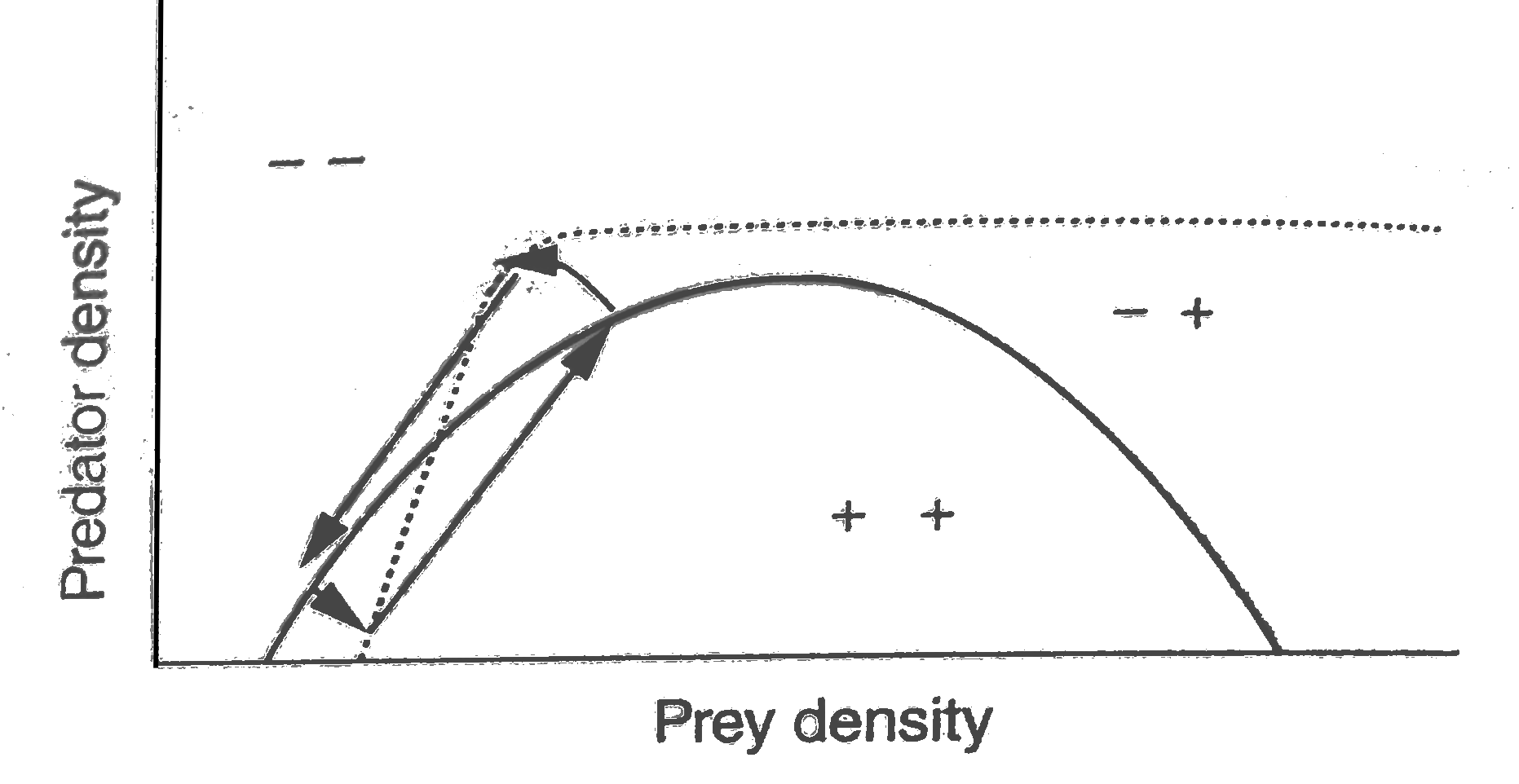 ] --- ## Stabilizing effect of refuge, graphically .pull-left-60[ 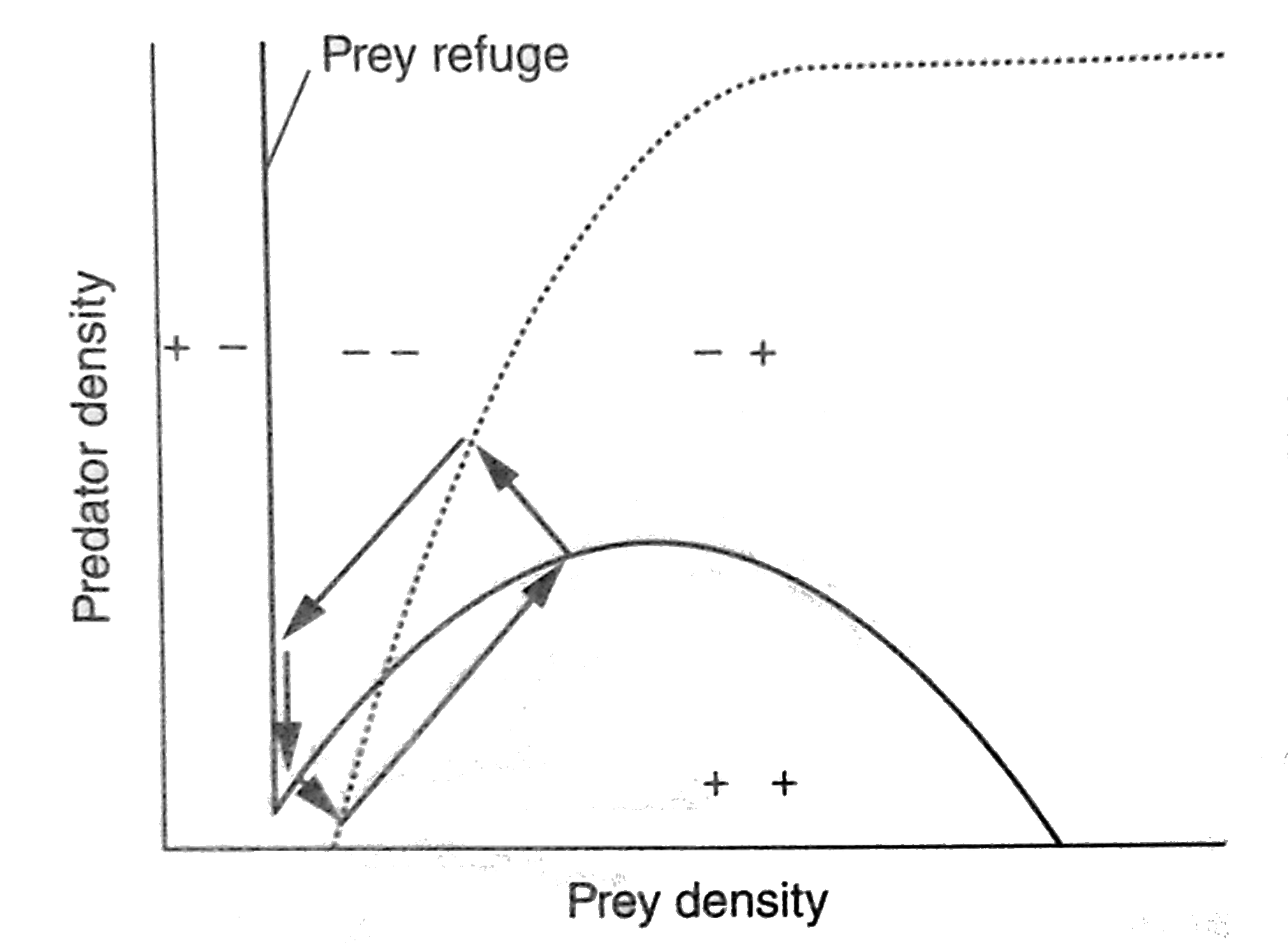 ] .pull-right-40[ .large[ A **refuge** is any area where there is **NO predation**. As long as there is *some* refuge, the oscillations are stabilized. ] ] --- ## Refuge effect .pull-left-30[ **Example:** Wildlife management "stumbled" in to this with wildlife reserves, the National Wildlife Refuge System, etc. On the one hand, people actively manage their land to attract game / fowl **enrichment**, on the other hand there are pockets where populations can always recover. ] .pull-right-70[ 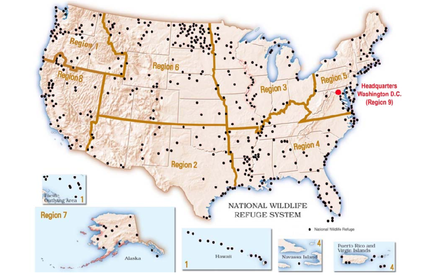 ] <!-- --- ## Embracing complexity: Jane Lubchenko .pull-left-40[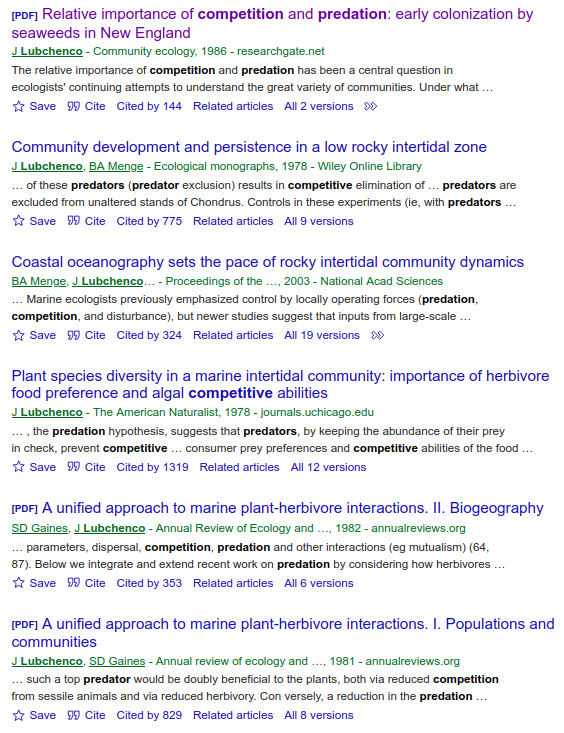] .pull-right[ Lots of fundamental, heavily cited papers on the relative roles of **predation**, **competition** and **external environmental effects** on intertidal rocky communities. .pull-right[  ] Later (2008-2016) secretary of National Ocean and Atmosphere Administration (NOAA). ] --> --- ## Introducing **Functional Response**... .center[ <img src="Interactions_PartIII_FunctionalResponses_files/figure-html/unnamed-chunk-4-1.png" width="80%" /> ] A **functional response** is the intake rate of a consumer as a function of food density. --- ## A more realistic functional response .pull-left[ <img src="Interactions_PartIII_FunctionalResponses_files/figure-html/unnamed-chunk-5-1.png" width="100%" /> ] .pull-right[ `$$f(V) = {aV \over 1+ahV}$$` Where `\(a\)` is attack rate, `\(h\)` is handling time. This assumes a single predator species focusing on a single prey species, getting slowed down by processing time. ] --- ## Holling's "disk" equation .pull-left[ 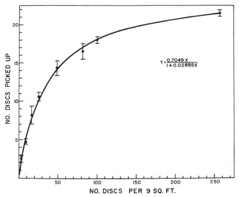 ] .pull-right[ An assistant picked sandpaper discs off a tackboard ([Holling 1951](https://doi.org/10.4039/Ent91385-7)). Fundamental foundations for predation theory ensued.  ] --- ## "Functional Response" keeps track of Prey Deaths ... .pull-left[ <img src="Interactions_PartIII_FunctionalResponses_files/figure-html/unnamed-chunk-6-1.png" width="100%" /> ] .pull-right[ ### Another functional response **Type III:** when prey are very scarce, there are other options for predators, or non-linear reasons why they're harder to find. ] --- ## Equally important .pull-left[ .large[to keep track of **Predator Response**] ] .pull-right-50[ <img src="Interactions_PartIII_FunctionalResponses_files/figure-html/unnamed-chunk-7-1.png" width="100%" /> ] --- ## Prey Response to Predation - **Total Prey Response** (V) = `\({\text{Prey eaten} \over \text{predator}} \times \text{predator response}\)` - **Prop. Prey Response** (V) = `\({\text{Total prey response} \over \text{Total prey}}\)` <img src="Interactions_PartIII_FunctionalResponses_files/figure-html/unnamed-chunk-8-1.png" width="100%" /> --- ## Prey deaths .pull-left[ <img src="Interactions_PartIII_FunctionalResponses_files/figure-html/unnamed-chunk-9-1.png" width="100%" /> ] .pull-right[ This curve (typically) peaks at some intermediate number, where: - (`1`) - N. Predators is (already) high, - (`2`) - N. of Prey consumed per Predator is high (approaching asymptote), but - (`3`) - Total N of prey is NOT too high. ] --- ## Prey growth All of that is total **mortality** of prey. Now - what we need is **proportional growth** of prey. We have a good, time-tested model for that: <img src="Interactions_PartIII_FunctionalResponses_files/figure-html/unnamed-chunk-10-1.png" width="100%" /> --- ## Combining **Growth** with **Removal** Where the two lines intersect, <font color = "darkorange"> **Growth** </font> = <font color = "purple"> **Removal** </font>, we're at equilibrium. The question is ... are these equilibria stable? .center[ <img src="Interactions_PartIII_FunctionalResponses_files/figure-html/unnamed-chunk-11-1.png" width="80%" /> ] --- ## Stability of equilibria Follow the arrows! .center[ <img src='timages/09_LookingForEquilibria.png' width='80%'/> ] **As usual, super elegant theory ... but what is it good for?** --- background-image: url("timages/MessierBackground.png") background-size: cover ## What limits moose? Big Q: Are herbivore populations controlled **bottom-up** (food limited) or **top-down** (predator limited). --- ## Models from theory .center[ <img src='timages/Messier1.png' width='80%'/> **Food regulates** ] --- ## Models from theory .center[ <img src='timages/Messier2.png' width='80%'/> **Food regulates, wolves limit (very slightly)** ] --- ## Models from theory .center[ <img src='timages/Messier3.png' width='80%'/> **2 equilibria! Either food or wolves regulate.** ] --- ## Models from theory .center[ <img src='timages/Messier4.png' width='80%'/> **Wolves definitely regulate.** ] --- ## Meta-analysis Data aggregated from many sites with high and low moose and wolf densities. .pull-left[ 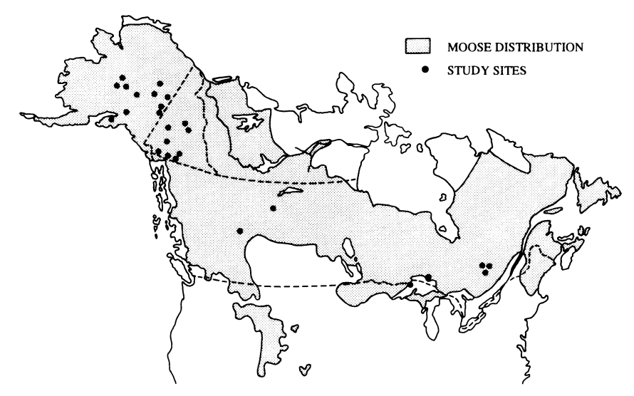 ] .pull-right[ 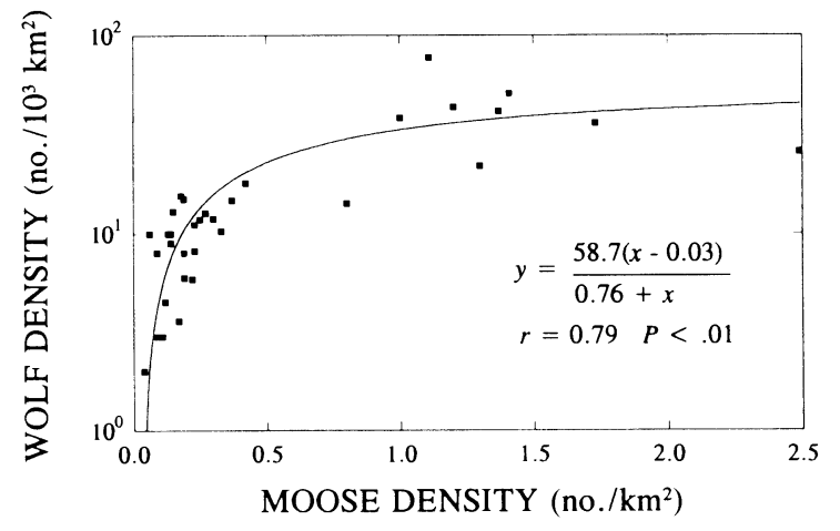 ] --- ## Empirically estimated ... .pull-left[ ### Functional response curve 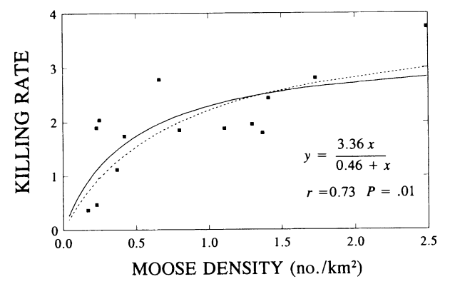 Looks Type II-ish, which makes sense since moose is (often) the main prey of wolves, and wolves are (often) the main predator of moose. ] .pull-right[ ### Density dependent growth curve 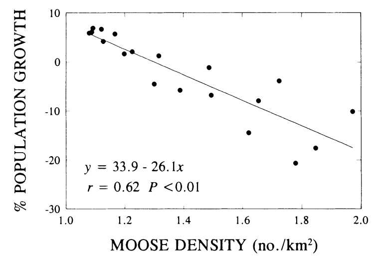 Note: these data are only from Isle Royale (Lake Superior) long term study. ] --- ## Put it all together ... .pull-left[ 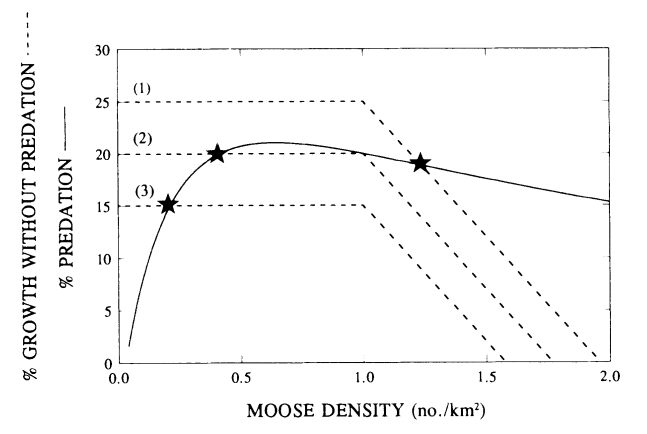 ] .pull-right[ - low productive environment (3) system more likely to be predator limited - more productive environment (1) more likely to be food-limited - a 2-state model is unlikely .... - ... but the numeric response curve is **shallow**. Meaning a local system (when perturbed) can switch from one to the other. - Consistent with observed variability not just in **space** but in **time**. ] --- class: inverse ## **Some major takeaways!** .pull-left.white.large[ 1. Ecological systems and populations can be EXTREMELY .lightred[**dynamic**] and .lightred[**complex**]! - This is a fundamental property of the evolutionary games of interaction: .yellow[production] / .yellow[consumption] / .yellow[competition] / .yellow[cooperation] that characterizes .lightgreen[**all life**]. 2. All models are **wrong** ... but **some** are useful. ] .pull-right[  ] --- class: inverse ## **Some major takeaways!** .pull-left.white[ ### **Well then what are models useful for?** .large[Mathematical models help us:] - .yellow[**explore**] and understand complicated systems (with math & simulations) - .yellow[**identify**] factors / dynamics / impacts that defy intuition - .yellow[**justify**] practical interventions for conservation and management .large[Statistical models help us:] - .orange[**design** and **plan**] how we make observations - .orange[**understand** and **interpret**] those observations ] .pull-right[  ] <!-- ## Proportional response of prey consumed is just the ratio: `\(P_v = f(V)/V\)` <img src="Interactions_PartIII_FunctionalResponses_files/figure-html/unnamed-chunk-12-1.png" width="100%" /> -->