class: center, top, title-slide .title[ # <strong>Population Ecology II: Limits on Population Growth</strong> ] .subtitle[ ## .white[EFB 390: Wildlife Ecology and Management] ] .author[ ### <strong>Dr. Elie Gurarie</strong> ] .date[ ### October 18, 2022 ] --- <!-- https://bookdown.org/yihui/rmarkdown/xaringan-format.html --> ## Estimating exponential growth rate from two points .pull-left-50[ 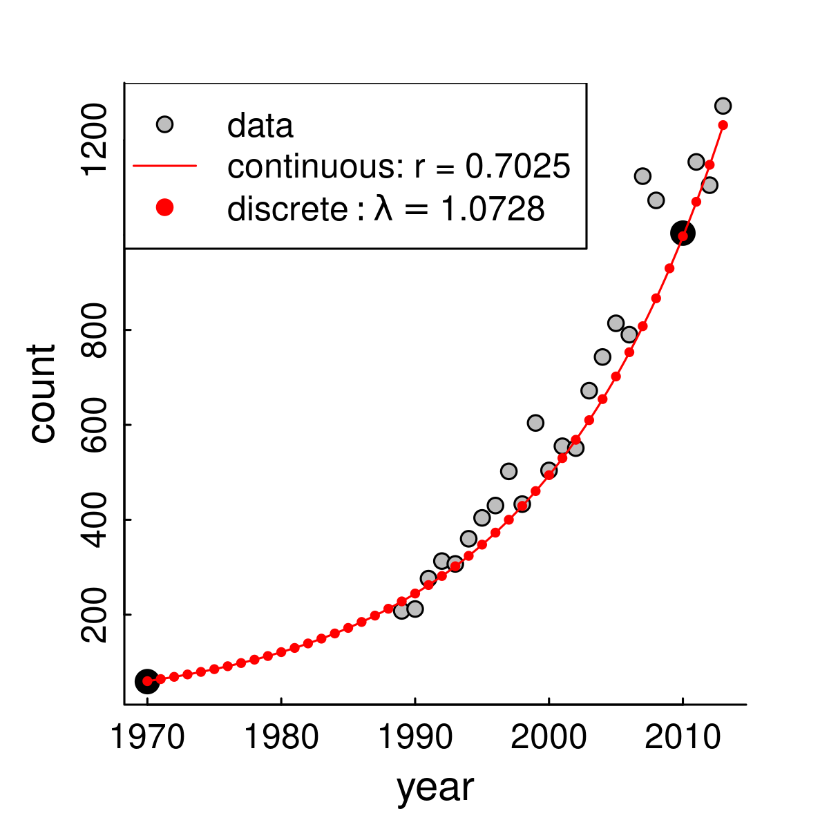 ] .pull-right[ We fitted this with just two points: year | N --|-- 1970 | 60 2010 | 1000 by solving for: `\(N_{2010} = N_{1970} \times \lambda^{(2010 - 1970)}\)` In a single formula: `$$\lambda = \exp\left( \frac{\log{N_t} - \log N_0 }{t} \right)$$` `\(\lambda = \exp (0.07) = \bf{1.0725}\)` 7.25% annual growth ] --- ## But you could/should use ALL the data! .pull-left[ **Using linear model of `\(\log(N)\)` to estimate growth rate** <!-- --> **Look how linear it's become!** ] .pull-right[ ### Population Growth model: `$$\large N_t = N_0 \lambda^t$$` ### Log of both sides: `$$\large \log(N_t) = \log(N_0) + \log(\lambda) \times t$$` this is a linear model! `$$Y = \alpha + \beta X$$` where `\(\large \widehat{\beta} = \log(\widehat{\lambda})\)` - so - `\(\large \hat{\lambda} = \exp\left(\widehat{\beta}\right)\)`] ] --- ## But you could/should use ALL the data! .pull-left[ **Using linear model of `\(\log(N)\)` to estimate growth rate** 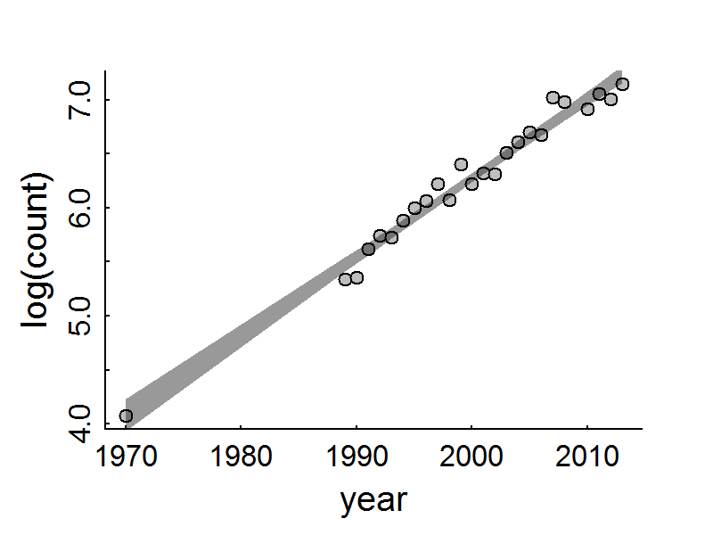<!-- --> **Look how linear it's become!** ] .pull-right[ ``` lm(log(count)~year, data = WA_seaotters) ``` Model output: .small[ <table> <thead> <tr> <th style="text-align:left;"> </th> <th style="text-align:right;"> Estimate </th> <th style="text-align:right;"> Std. Error </th> <th style="text-align:right;"> t value </th> <th style="text-align:right;"> Pr(&gt;|t|) </th> </tr> </thead> <tbody> <tr> <td style="text-align:left;"> (Intercept) </td> <td style="text-align:right;"> -140.2227 </td> <td style="text-align:right;"> 4.7318 </td> <td style="text-align:right;"> -29.6344 </td> <td style="text-align:right;"> 0 </td> </tr> <tr> <td style="text-align:left;"> year </td> <td style="text-align:right;"> 0.0733 </td> <td style="text-align:right;"> 0.0024 </td> <td style="text-align:right;"> 30.9533 </td> <td style="text-align:right;"> 0 </td> </tr> </tbody> </table> ] **Using ALL THE DATA, we get the benefit of a precision estimate as well:** `$$\widehat{\lambda} = \exp(\widehat{\beta});\,\, \widehat{\lambda} = 1.076 \pm 0.005$$` .green.small[(actually, 95% confidence interval is not quite symmetric: `$$\small \exp(\widehat{\beta} - 2\sigma_{\beta}), \exp(\widehat{\beta} + 2\sigma_{\beta})$$` but close enough)] ] --- .pull-left-60[ ## Sources of variation? 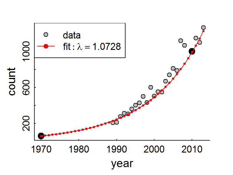<!-- --> ] ### Observation error. - How **precise**/**accurate** is the actual estimate? -- ### Unexpected immigration / emigration. - check assumptions about "closed population" -- ### .red[**Environmental Stochasticity**] Environment good / bad affecting **birth** and **death** for all animals. --- .pull-left[ ## Demographic Stochasticity .darkred[**Stochasticity**] means: **randomness** in **time**. ***Demography*** is the **Science of Population Dynamics**. Often it refers specifically to **births** and **deaths** (and **movements** ... but we're still looking at closed population). Individually, *all* demographic processes are stochastic. An individual has some **probability** of dying at any moment. An individual has some *probability* of reproducing (or some probability distribution of number of offspring) at a given time. .green[**Question:**] How important is the randomness of *individual* events for a *population* process? .green[**More specific Q:**] What is the probability of extinction? ] -- .pull-right[ ## Human Experiment .red[ > - 15 students > > - Flip a survival coin. > > - If you die (tails) sit down, if you live (heads) stay standing > > - Flip a reproduction coin. > - If you reproduce (heads) call on another student to stand ] ] --- ## Cranking this experiment very many times. .pull-left[ https://egurarie.shinyapps.io/StochasticGrowth/ 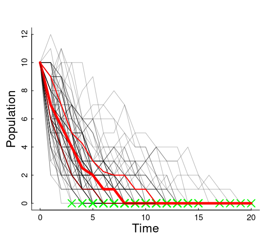 ] .pull-right[ On average, the number of individuals at time `\(t+1\)` is the number that survived + the number that reproduced of those that survived. `$$E(N_{t+1}) = p_s N_t + p_b\,p_s N_t = p_s (1+p_b) N_t$$` So (in our coin flip example) `$$\widehat{\lambda} = p_s (1+p_b) = 0.75$$` **What does that mean for our population!?** .center.large.red[Extinction is inevitable!] ] -- --- ## Even when population growth is 0... .pull-left-60[  ] .pull-right-40[ Even if the population growth is 0 (neither growing nor falling) .... `$$\widehat{\lambda} = 0.5 \times (1+1) = 1$$` **demographic stochasticity** leads to *some* probability of extinction always. ### Main take-away **Demographic stochasticity** is important only for *small* populations. ] --- ## Environmental Stochasticity .pull-left-30[ - Affects entire population - Can ALSO increase risk of extinction - or at least drive populations ] .pull-right-70[  ] .pull-left-70[ --- ## As populations grow ... ### they always hit **Limits to growth** .content-box-blue.large[ - Space limits - Resource limitations - Competition - Predation - Disease *All of these can interact * ] ] .pull-right-30[  ] --- ## Fundamental population equation `$$\huge \Delta N = B - D + I - E$$` .large[ Exponential growth assumes these (especially .red[**Birth**] & .red[**Death**]) are proportional to .red[**N**]. But at high N ... B can fall, or D can rise, or I can decrease or E can increase. ] ### Density dependence .large[ Means that the *rate* of a parameter(e.g. `\(b = {B\over N}\)` or `\(d = {D\over N}\)` is: - (a) NOT constant - (b) dependent on total population (or density) `\(N\)`. ] --- .pull-left-50[ ## Example: Wolf populations - Dispersal into new area, mainly wolf mating pairs. - Highly territorial! - Wolves produce up to 4 pups per litter that survive - If there are no neighbors, wolves will disperse to found new packs - Pack with 8 adults or 2 adults, still produces (about) 4 pups per litter - If there are lots of neighbors, packs become larger (more individuals) in smaller territories. <img src='images/WI_WolfTerritorySize.png' width='80%'/> ] .pull-right-50[ **Expansion of Wisconsin Wolves, 1970's to 2000's**  ] --- ## Human-wolf experiment model .pull-left-60[ ### basics of model - 8 possible territories - 1 initial dispersing wolf (female) ### each season ... - One female / pack gives birth to 2 offspring - Offspring can choose whether to disperse or not - 1/4 of all wolves die each year ] .pull-right-40[ 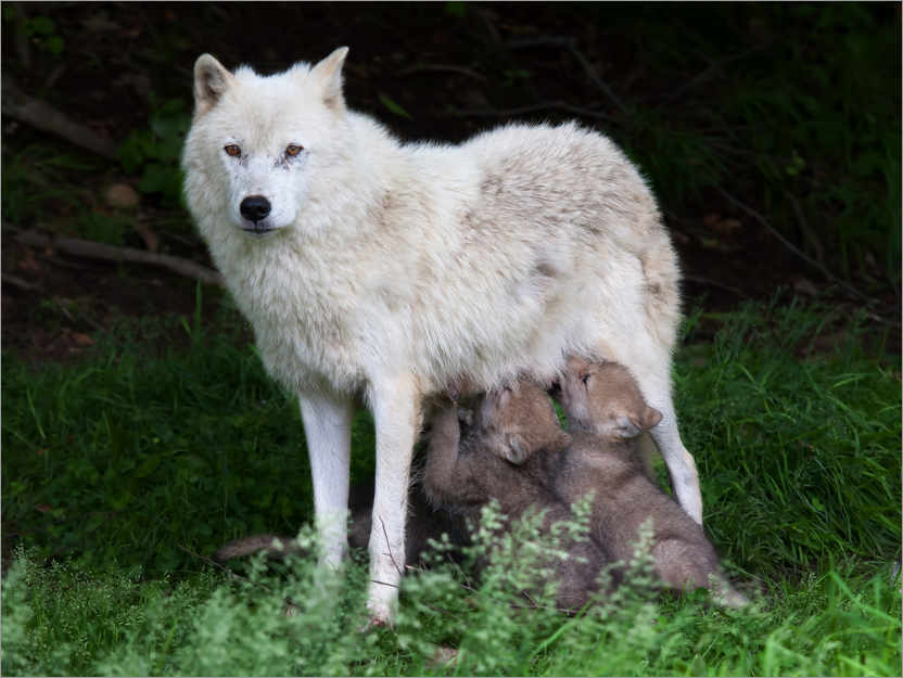 ] Enter data [here](https://docs.google.com/spreadsheets/d/15j2b3FCfbtrPkAlRb6QE6s55aRqggeSDi5YU6OBh7Yc/edit?usp=sharing) --- class: inverse ## Results of Human Wolf Experiment .center[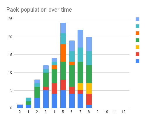 Looks a lot like initial exponential growth stabilizes around 20 ind as die-offs balance out births. ] --- .pull-left[ # Modeling wolf population Population equation: `$$N_t = (1 + b - d) \times N_{t-1}$$` Death rate is constant: `\(d = 0.25\)` Birth rate is high when population is low: `\(b_0 = 2\)` Birth rate is small when population is high: - `\(N = 1\)`; `\(B = 2\)`; `\(b = 2\)` - `\(N = 8\)`; `\(B = 16\)`; `\(b = 2\)` But it hits an absolute maximum of 16 total. So if: - `\(N = 32\)`; `\(B = 16\)`; `\(b = 1/2\)` - `\(N = 64\)`; `\(B = 16\)`; `\(b = 1/4\)` ] .pull-right-40[ <!-- --> ] --- .pull-left-60[ ## Some Concepts - Natural populations are always eventually limited - The "cap" on a population is called the .darkred[***Carrying Capacity*** ] (symbol: **K**). This is - When population rates (*b*, *d*, also *i*, *e*) depend on the **total population**, this is called: .darkred[***Density Dependence***]. - The maximum growth rate (max `\(b-d\)`) is called the .darkred[**intrinsic growth rate**]. ] .pull-right-40[ 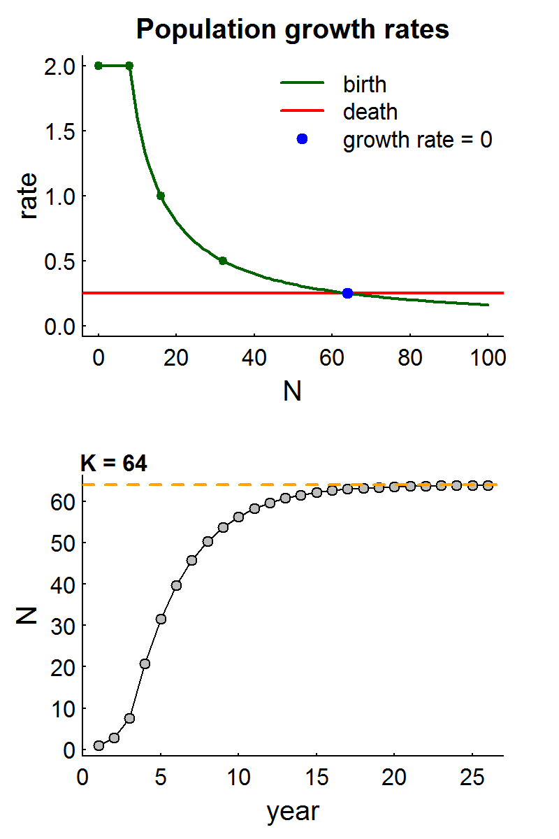<!-- --> ] --- .pull-left[ # Logistic growth .darkred[***Logistic growth***] is a specific kind of .darkred[Density Dependent] growth where the relationship between ***r*** and ***N*** is .darkred[**linear**]. The formula is: `$$r = r_0 (1 - N/K)$$` <img src="Lecture_PopulationEcology_PartII_files/figure-html/unnamed-chunk-9-1.png" width="100%" /> ] .pull-right[ 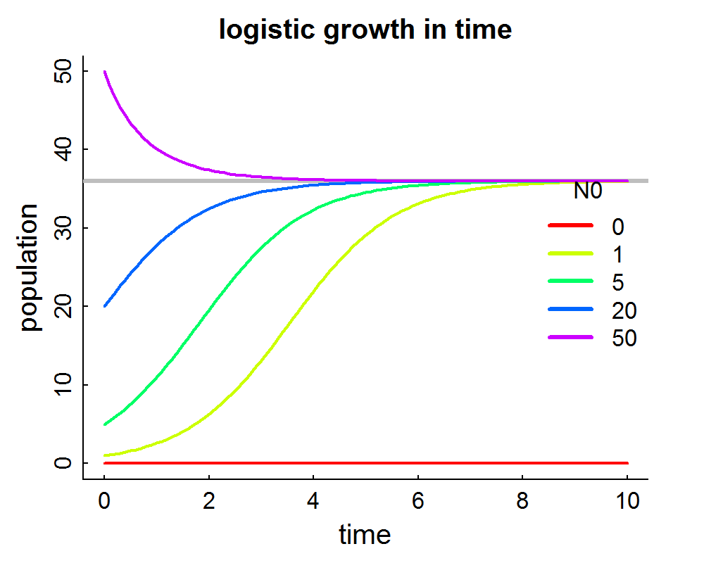<!-- --> - At `\(N=0\)` - growth = 0 - At `\(N\)` slightly above 0 - growth maximum `\(\approx r_0\)` - At `\(N = K\)` - growth = `\(0\)` - At `\(N > K\)` - growth < `\(0\)` ] --- .pull-left-40[ ## Intrinsic growth rates Strong Relationships with body size: .large[ `$$\large r_0 = 1.5 \, W^{-0.36}$$` ] `\(W\)` is live weight in kilograms **Q. Why would this be the case?** ] .pull-right-60[  .center[Fryxell chapter 6] ] --- ## Different models of density dependence .pull-left-30[ **What is it that depends on density?** Is it birth? Is it death? Is it linear? Is it curvy? ] .pull-right-70[  .center[Fryxell chapter 8.] ] --- ## Density dependent mortality & fecundity .pull-left-30[ - Calf / pup / juvenile mortality is highest when densities are highest. - **Fecundity** (# of offspring per female) falls at high densities. - This effect mainly kicks in at very high numbers (not linear). ] .pull-right-70[  .center[Fowler (1981)] ] --- .pull.left[ ## Concave curves: Butterflies ] .pull-right[Note that the **density dependent effects** kick in when populations are **small** rather than **large**.]  .center[(Nowicki et al. 2009)] --- ## Carrying capacity .pull-left[ **Ecological carrying capacity** Basically - *K* of a logistic growth Limited (almost always) by: - resources: - food - shelter - breeding **habitat** - space - interactions (predation / parasites / disease) ] .pull-right[ > For the **Howework assignment** you will explore different ways in which **Carrying Capacity** is estimated, and why it is an important question for wildlife ecologists to ask. ] --- ## Some references .small[ - Benton, T. G., A. Grant, and T. H. Clutton-Brock. 1995. Does environmental stochasticity matter? Analysis of red deer life-histories on Rum. Evolutionary Ecology 9:559–574. - Chapman, E. J., and C. J. Byron. 2018. The flexible application of carrying capacity in ecology. Global Ecology and Conservation 13:e00365. - Fowler, C. W. 1981. Density Dependence as Related to Life History Strategy. Ecology 62:602–610. - Laidre, K. L., R. J. Jameson, S. J. Jeffries, R. C. Hobbs, C. E. Bowlby, and G. R. VanBlaricom. 2002. Estimates of carrying capacity for sea otters in Washington state. Wildlife Society Bulletin:1172–1181. - McClelland, C. J. R., C. K. Denny, T. A. Larsen, G. B. Stenhouse, and S. E. Nielsen. 2021. Landscape estimates of carrying capacity for grizzly bears using nutritional energy supply for management and conservation planning. Journal for Nature Conservation 62:126018. - Nowicki, P., S. Bonelli, F. Barbero, and E. Balletto. 2009. Relative importance of density-dependent regulation and environmental stochasticity for butterfly population dynamics. Oecologia 161:227–239. - Potvin, F., and J. Huot. 1983. Estimating Carrying Capacity of a White-Tailed Deer Wintering Area in Quebec. The Journal of Wildlife Management 47:463. - Sibly, R. M., D. Barker, M. C. Denham, J. Hone, and M. Pagel. 2005. On the Regulation of Populations of Mammals, Birds, Fish, and Insects. Science 309:607–610. - Thébault, J., T. S. Schraga, J. E. Cloern, and E. G. Dunlavey. 2008. Primary production and carrying capacity of former salt ponds after reconnection to San Francisco Bay. Wetlands 28:841–851. - Wydeven, A. P., T. R. Van Deelen, and E. J. Heske, editors. 2009. Recovery of Gray Wolves in the Great Lakes Region of the United States: An Endangered Species Success Story. Springer New York, New York, NY. ]