class: top, left, title-slide .title[ # .white[Mark-Recapture and Index Counts] ] .subtitle[ ## .white[EFB 390: Wildlife Ecology and Management] ] .author[ ### .white[Dr. Elie Gurarie] ] .date[ ### .white[September 18, 2025] ] --- class: inverse <!-- https://bookdown.org/yihui/rmarkdown/xaringan-format.html --> ## Mark-Recapture .pull-left[ .large[is a super-versatile, very common tool for: - **Estimating Abundances** (with confidence intervals) ... But also: - Survival - Growth Rate - Reproductive Rates ]] .pull-right[ 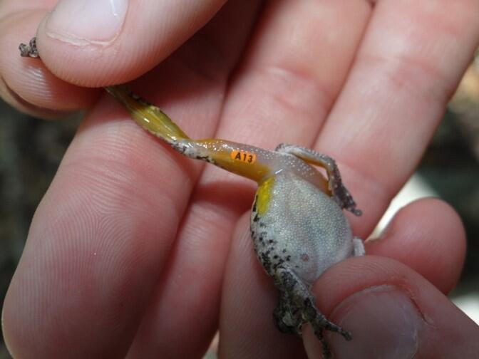 [USGS Bayou Treefrog Project](https://www.usgs.gov/centers/wetland-and-aquatic-research-center/science/capture-mark-recapture-treefrogs-bayou-teche) ] --- class: inverse ## How!? 1. Capture individuals at time `\(t\)` - In their reproduction area, their wintering area, along their migration route… - using traps, nets, anesthesia, binoculars 2. Mark `\(M\)` individuals - Using paint, ring, tag, collar, chip, transponder… 3. Release the individuals at the capture site 4. Re-capture `\(C\)` individuals at time `\(t+1\)` - Physically or visually - In the same area of the first capture either the same year or the next one 5. Count the marked individuals `\(R\)` in the new subset --- ## Mark-Recapture is Super Simple 1. mark random subset, 2. release, 3. recapture, 4. count marked  --- ## Mark-Recapture .squeeze-70[ Basic idea, **ratios should be similar**: `$${marked\,(M) \over total\,(N)} = {recapture\,marked (R) \over recapture\,total (C)}$$` ] --- ## Mark-Recapture .squeeze-70[] .pull-left.center[ Convert that to estimate: `$$\widehat{N} = {𝑀 \times 𝐶\over 𝑅}$$` **Lincoln-Petersen Index** ] -- .pull-right.center[ And there's a formule for SE `$$SE(\widehat{N}) = \sqrt{M^2(C+1)(C-R)\over{(C+1)^2(C+2)}}$$` ] --- ## Challenges: .center.large[Delineating the spatial limits of the ***“population”***] ### Sometimes easy! 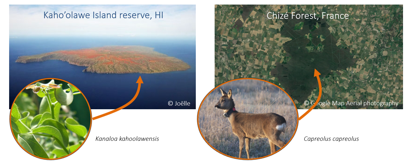 --- ## Challenges: .center.large[Delineating the spatial limits of the ***“population”***] ### Sometimes hard! .squeeze-70[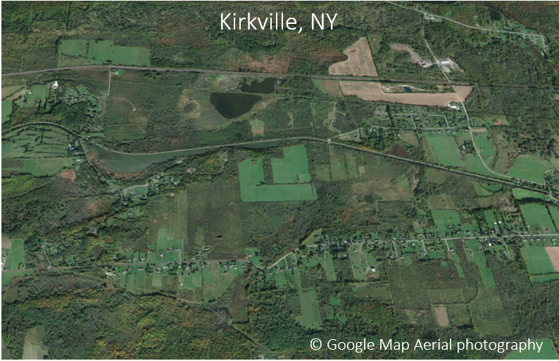] --- ## Challenges: .center.large[Choosing a minimally harmful method of **capture**] 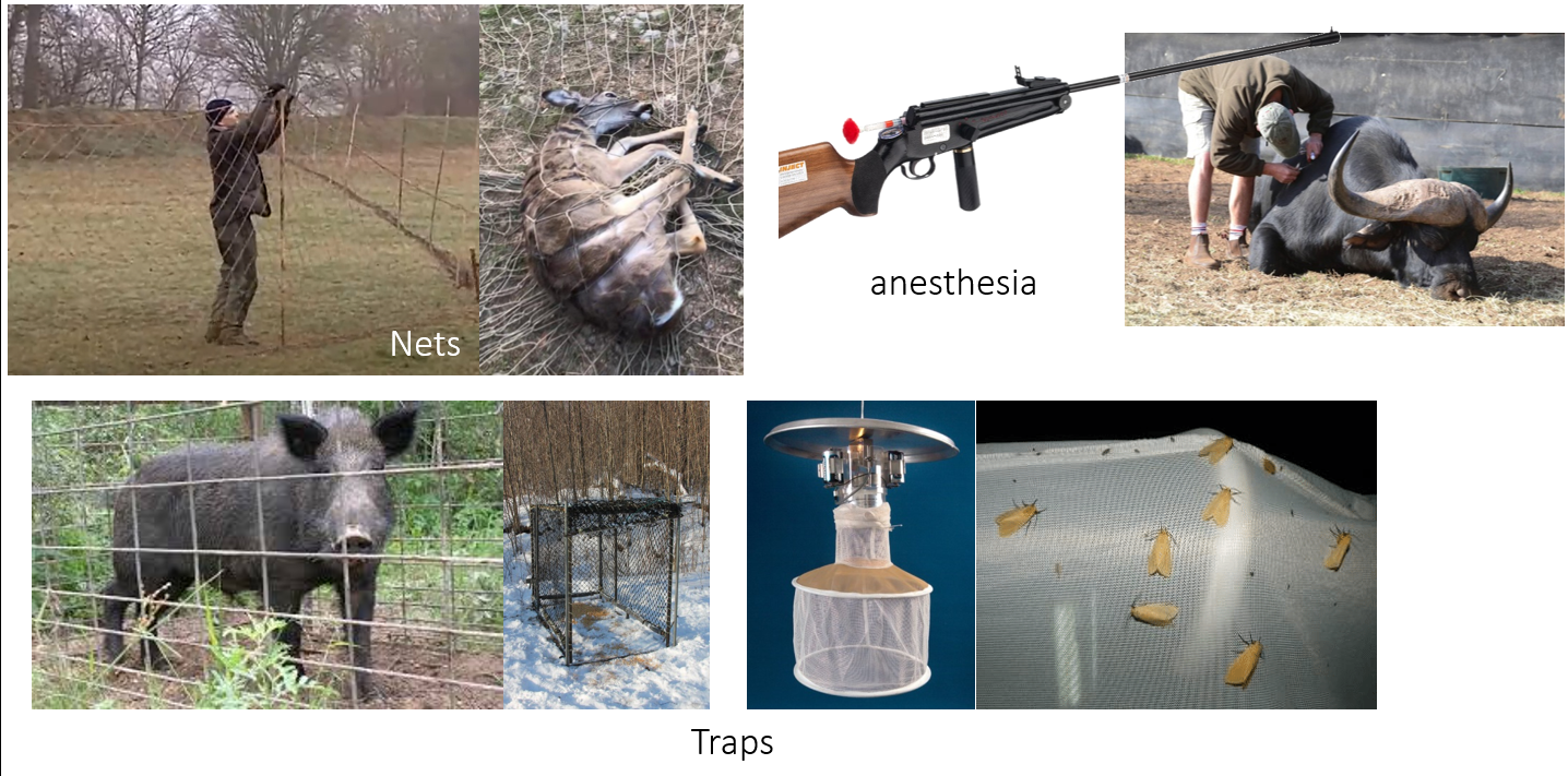 --- ## Challenges: .large[**Best:** (but limited in practice) is **Visual Capture** (and recapture)] .pull-left-40[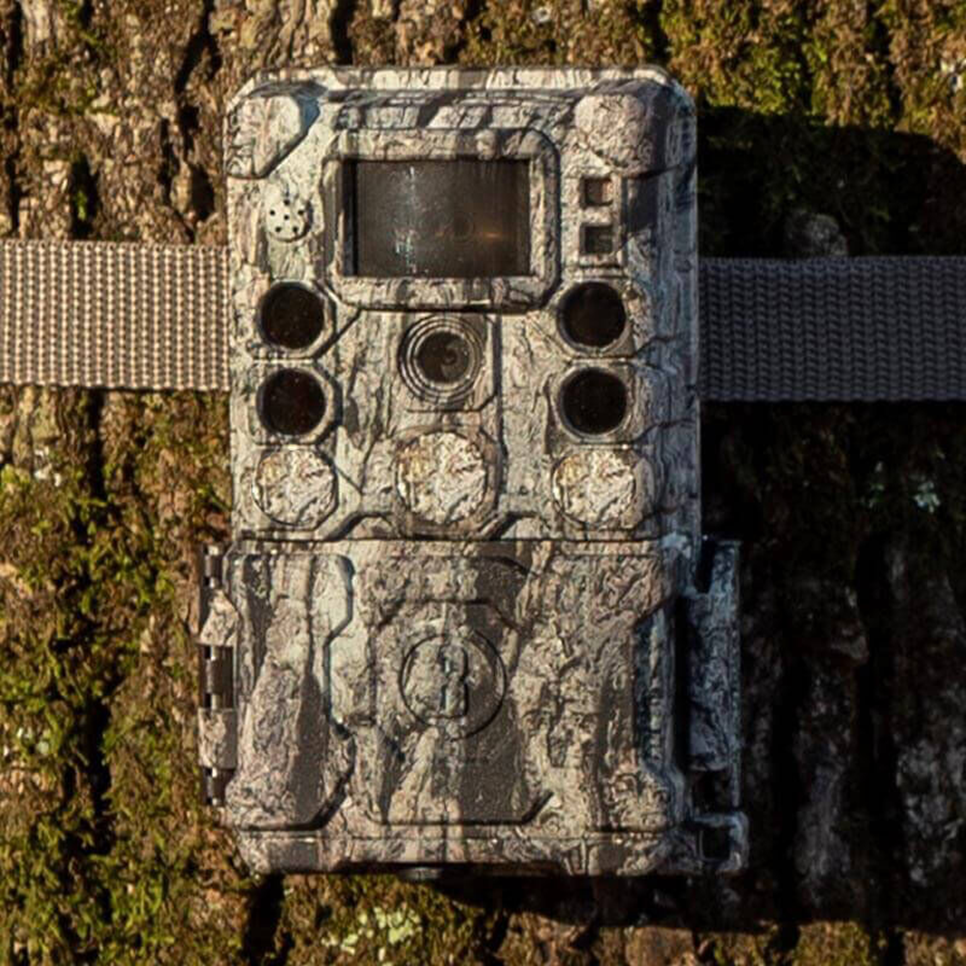] .pull-right-60[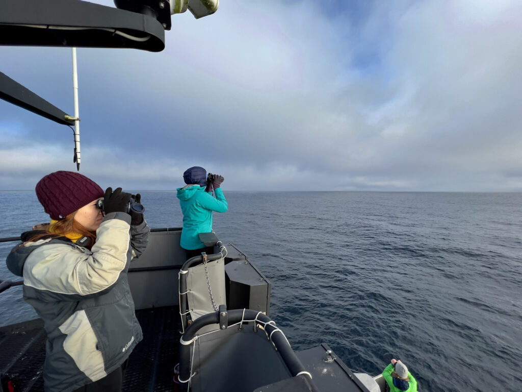] --- ## Challenges: .center.large[Choosing a minimally invasive method of **marking**] 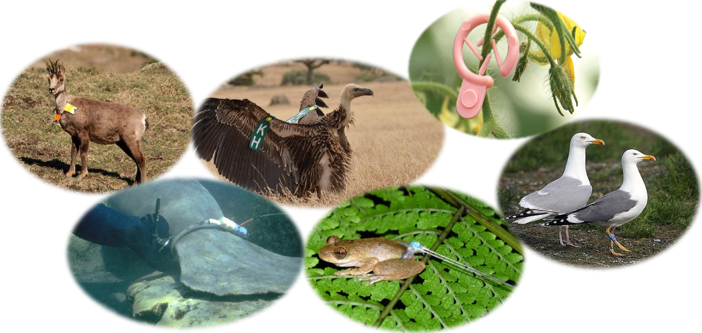 --- ## Challenges: .center.large[Choosing a minimally invasive method of **marking**] 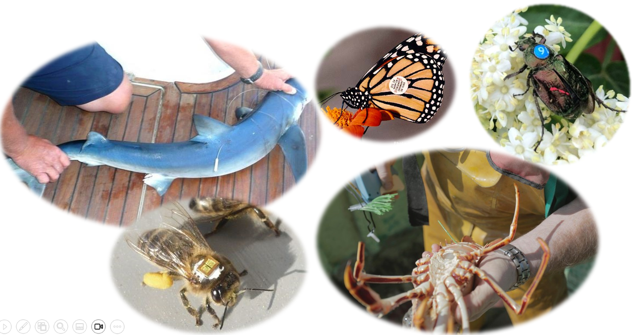 --- ## Challenges: .large[**Best:** (but limited in practice) is **Visual Capture** (and recapture)] 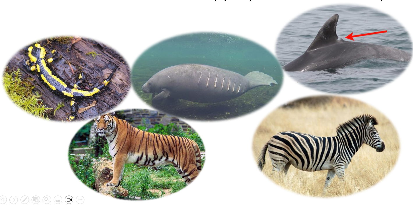 --- class: inverse ## I banded students! .pull-left-50[  ] .pull-right-50.center[ ... by going back in time and subtly manipulating your parents so that exactly .Large.red[**M<sub>t</sub> = 27**] of you have the letter .Large.red[**O**] in your first name. ] --- ## How many O's? .pull-left.large[ You have **5 minutes** to survey as many students in the class as you can (but not more than 20). Ask whether they have an .red[**"O"**] in their last name. Count yourself! Report your results here: Remember, your sample should be **random**! (*do not seek out 'O's*). ] .pull-right[  https://forms.gle/JpVNNjxpsHcTRM3a9 ] --- class:center, inverse ## Pause to compute the results  .pull-left[$$\large \widehat{N} = {𝑀 \times 𝐶\over 𝑅}$$] .pull-right[$$SE = \sqrt{M^2(C+1)(C-R)\over{(C+1)^2(C+2)}}$$] --- ## Important assumptions of the Lincoln-Petersen Index .large[ 1. No deaths | no births 3. No immigration | no emigration 5. Random and equal probability sampling of marked and unmarked 5. No marks get lost **Do these assumptions hold for the Great Banded Student Count?** ] --- ## But when they don't hold and if you go deep into statistical methods, you can learn a lot... -- for example about Steller sea lions (*Eumetopias jubatus*). 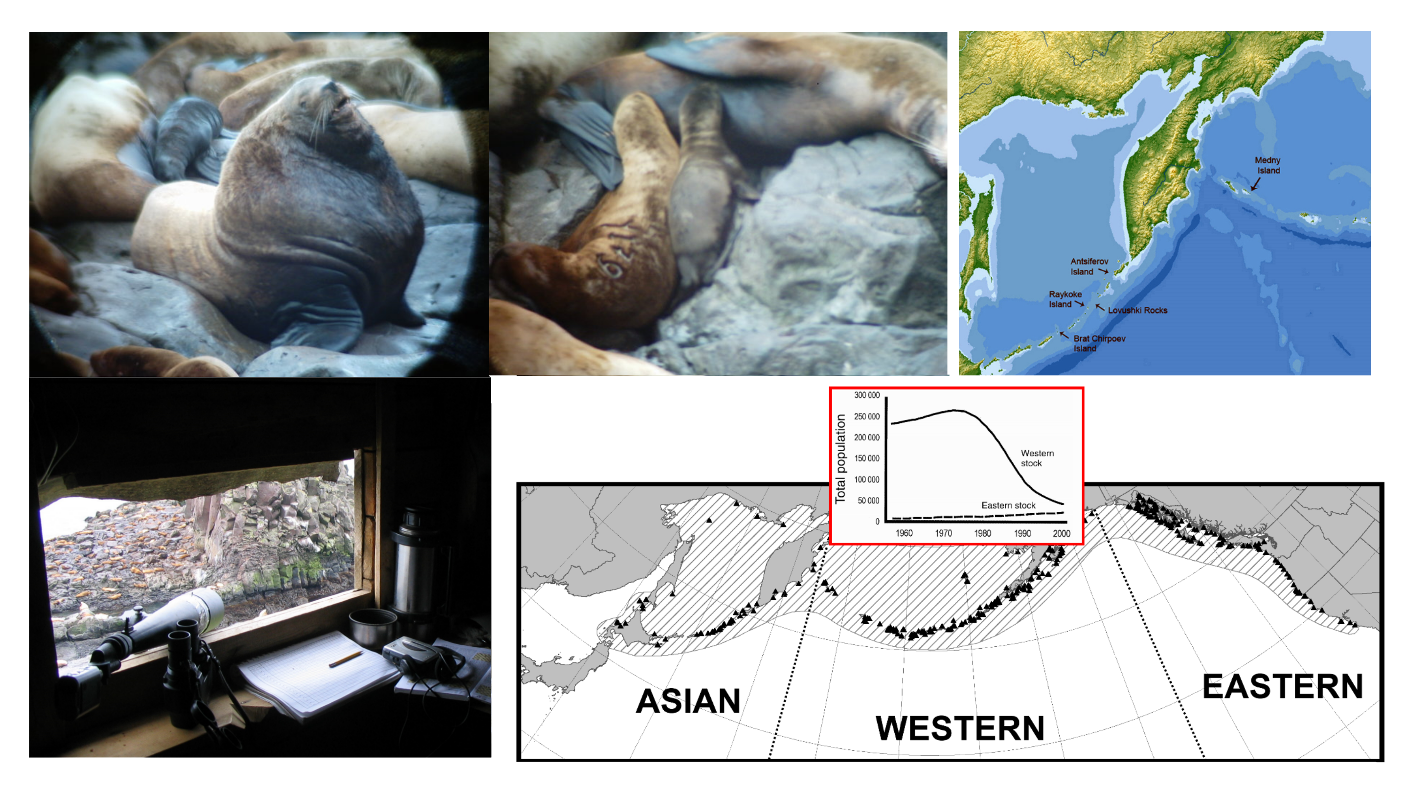 --- .pull-left[.content-box-blue[#### Mark-recapture study (since 2004) - `\(>\)` 200,000 - daily resights - `\(>\)` 4,765 animals - all photo controlled - `\(>\)` 40,000 - photos of marked animals ]] .pull-right[.content-box-green[#### Estimates of: - Survival - Reproduction rates - Migration ] **AFAIK - the best age-specific vital rates of any large mammal**. ] 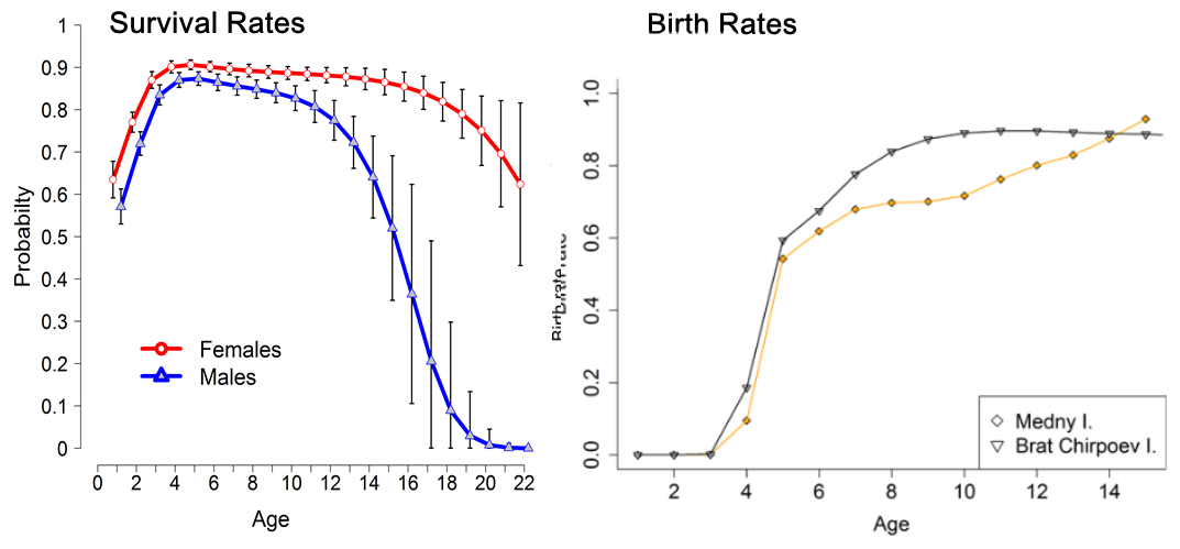 .center[[Altukhov, A. et al. (2015) PLoS One 10(5):e0127292](https://journals.plos.org/plosone/article?id=10.1371/journal.pone.0127292)]] --- class: ## Non-invasive mark-recapture <iframe src="https://www.youtube.com/embed/P9H-S7pMOf4?controls=0" width="900px" height="500px"> </iframe> --- background-image: url('images/noninvasive.png') background-size: cover ## Non-invasive mark-recapture - Visual identification of natural markings - Camera traps - Binoculars - Fur snags - (**genetic mark-recapture**) - Fecal samples - (**genetic mark-recapture**) --- ### Example of estimates based on genetic mark-recapture .pull-left-40[ 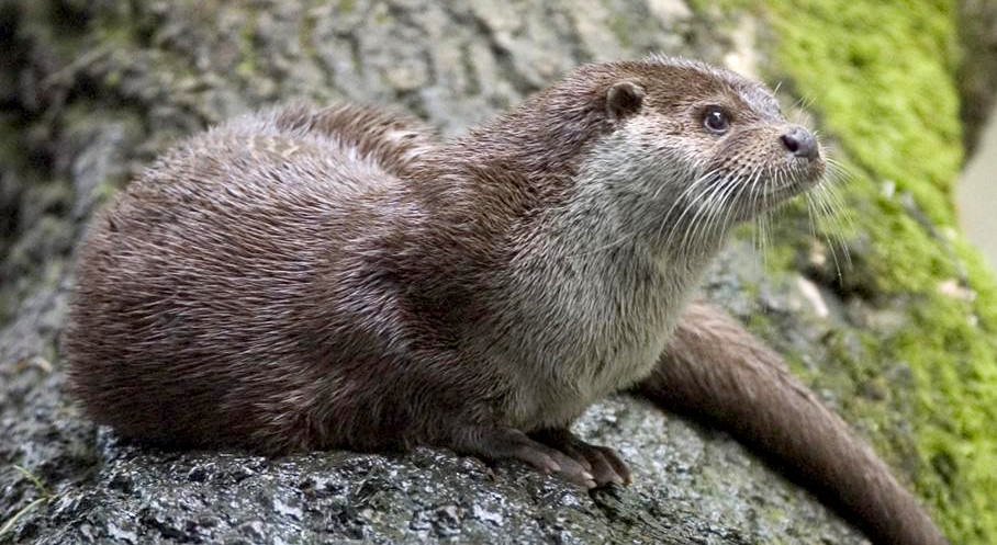 Eurasian otter (*Lutra lutra*). Elusive, aquatic, nocturnal. Deposits: ***spraint*** ] -- .pull-right-60[ 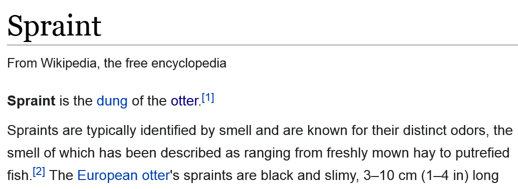 ] --- -- .pull-left-40[ **Methods:** 1. Collect spraint 2. Genotype microsattelites - those are the marks 3. Recapture (of spraint) proceeds as before ] .pull-right-60[ .blockquote[.blue.small[*Using 2132 otter faeces of a wild otter population ... collected over six years (2006–2012) ... We provide precise population size estimate with confidence intervals (for 2012: `\(\widehat{N} = 20 ± 2.1\)`, `\(95\%\, \text{CI} = 16–25\)`)* .center[[(Lampa et al. 2015, PLOS)](https://journals.plos.org/plosone/article?id=10.1371/journal.pone.0125684)]]] ] --- background-image: url('images/scat.jpg') background-size: cover ## .white[**Index counts**] --- class:inverse ## Index counts are indirect observations which can be *related* to total abundances OR which can be useful for detecting trends / comparisons where you don't care (or can't get) absolute abundances. Examples: - Bird calls - Nest counts - Roost counts - Animal tracks - Fecal counts 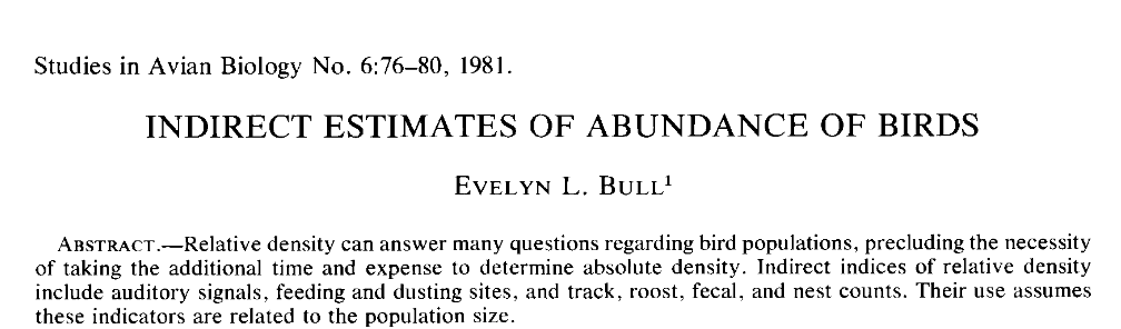 --- ## Fecal counts <iframe src="https://www.youtube.com/embed/n3YbcoTMQzk?controls=0"z width="800px" height="450px"> </iframe> --- ## Index-manipulation-index method 1. Obtain one index of population size: `\(I_1\)` 2. Remove a bunch of animals `\(C\)` 3. Obtain another index of population size: `\(I_2\)` -- Then ... `$$\widehat{N_1} = {I_1 C \over I_1 − I_2}$$` `$$SE = \widehat{N_1} {q^* \over p^*} \sqrt{{1 \over I_1} + {1 \over I_2}}$$` - `\(p^*\)` is proportion removed: `\(I_1 - I_2 \over I_1\)` - `\(q^*\)` is proportion remaining: `\(1 - p^*\)` -- .content-box[**Very important assumption:** Closed population, i.e. no births / deaths / emigration] --- ## Feral horse - fecal index + cull + fecal index .pull-left-30[ .red[ #### Data: `\(I_1 = 301\)`; `\(I_2 = 76\)` `\(C = 357\)`; `\(p* = 0.748\)` ] ] .pull-right-70[ 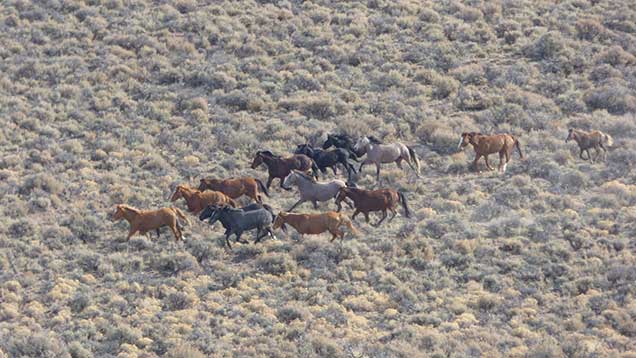 Feral horses - Beaty's Butte, Oregon ] .blue[ #### Estimates: `\(\widehat{N_1} = (301 × 357)/(301 − 76) = 478\)` with standard error: `\(SE(\widehat{N_1}) ≈ 478\times(0.252/0.748)\times\sqrt{(1/301 + 1/76)} = 21\)` ] .center[(see: [Eberhardt 1982](https://www.jstor.org/stable/pdf/3808648.pdf))] --- # North American Breeding Bird Survey Based mainly on volunteer expert birder detection of male breeding songs.  --- # North American Breeding Bird Survey Good for identifying large-scale trends ... but hard to get abundance estimates: .center[ <img src="images/shrike.jpg" width="70%" /> ] --- ## Counting tracks Used widely in Russia and Finland in standardized, repeated, long-term random transects. **Method:** ski, and count (and ID) every track you cross .pull-left-40[ 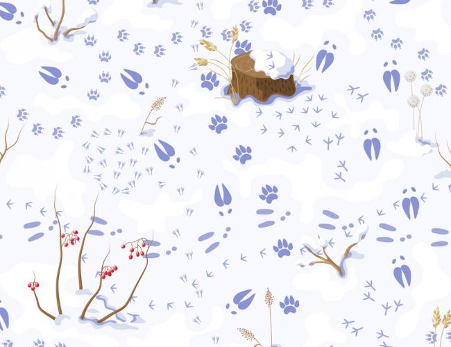 ] .pull-right-60[ Conversion to density estimate: **Formozov–Malyshev–Pereleshin** (FMP) `\(\widehat{D} = {\pi \over 2} {x\over S \hat{M}}\)` where: - *x* - number of track crossings - *S* - transect length - *M* - animal movement length Very simple, surprisingly effective. ] --- .pull-left-30[ <img src="images/wildlifetriangle.jpeg" width="90%" /> 4 km / side x 3 Note intense coverage! <img src="images/finland.jpeg" width="80%" /> ] .pull-right-70[ ## Finland Wildlife Triangles 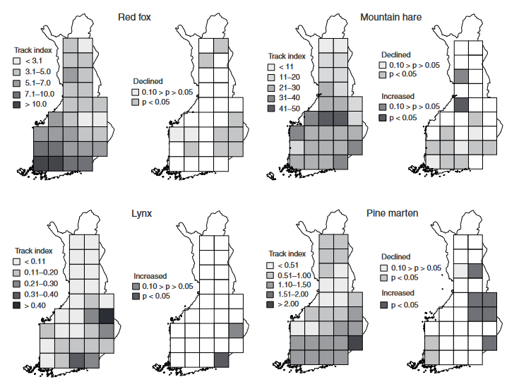 ] Detecting trends, and inferring predator-prey interactions. ([Kauhala and Helle 2000](https://www.jstor.org/stable/23735998)) --- ## Large-scale patterns 50,000 transects between 1950-2010 .pull-left[ 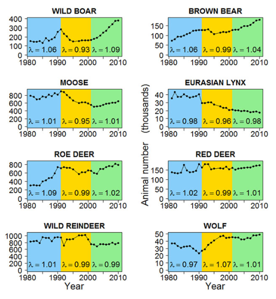 ] .pull-right[ **Moose trends** 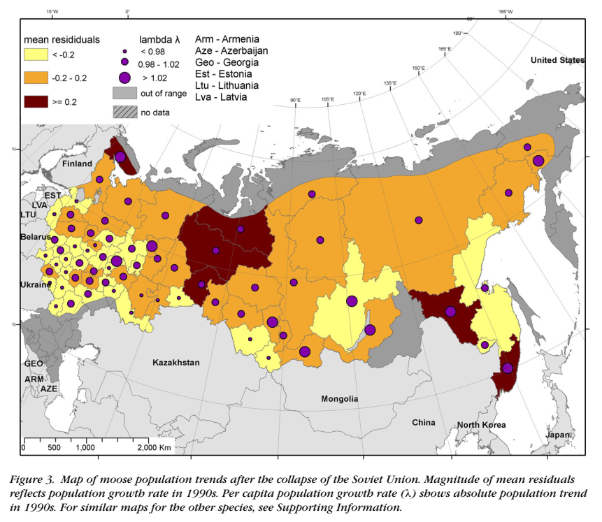 ] Reveal impact of socioeconomic upheaval on wildlife. ([Bragina et al. 2015](https://www.jstor.org/stable/23735998)) --- ## Kalahari Tracking-Based Density Estimation .pull-left-30[ FMP formula: `\(\Large \widehat{D} = {\pi \over 2} {x\over S \widehat{M}}\)` ] .pull-right-70[ 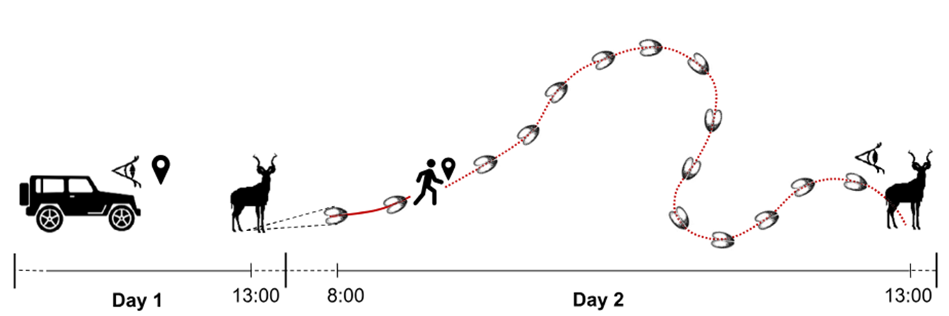 ] <br> .center[ Big Question: ***What is daily movement rate *** `\(\widehat{M}\)` ? ] <br><br> .pull-left-40[] .pull-right-60[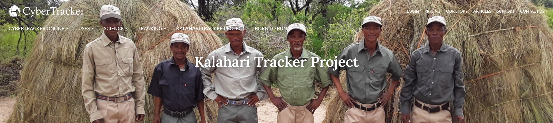] <br><br> ([Gielen et al. 2025](https://www.jstor.org/stable/23735998)) --- ## Kalahari Tracking-Based Density Estimation .pull-left-40[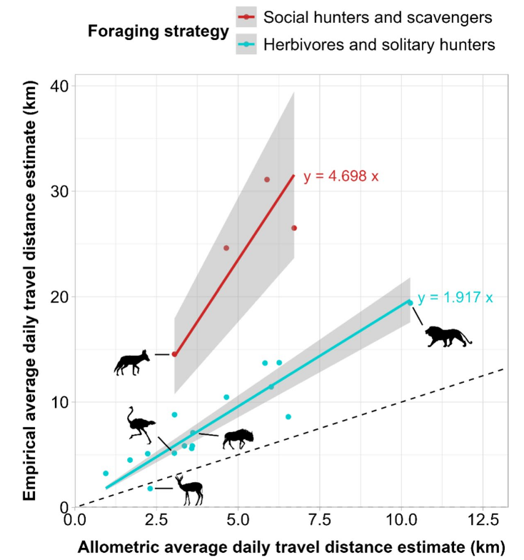 .small[Field based tracking of lots of species, filling in the gap with linear models...] ] -- .pull-right-60[ 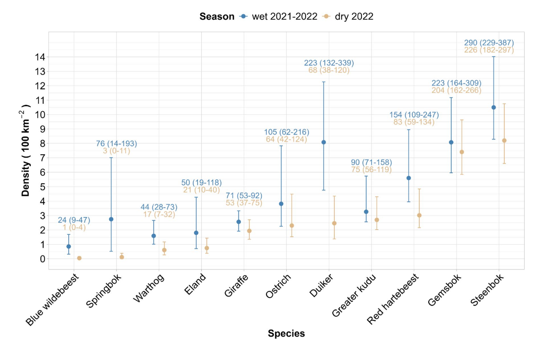 can be converted to density Estimates (with confidence intervals of course)! ] -- .darkred[***Elegant combination of Indigenous Knowledge, non-invasive techniques, and some sneaky math to get density estimates.***] --- ### Take-aways .blockquote[ Thinking about **abundance estimation** helps us think about: (a) tools for oberving and monitoring wildlife, (b) creative ways to make inferences about wildlife, (c) some of the sources of randomness and variability that characterize *ALL* observations of wildlife. ] <br> .pull-left-30[ .content-box-yellow[ **Total counts** - expensive - hard - possible for few animals **Sample counts** - involve stats and good design - possible for more animals ] ] .pull-right-70[ .content-box-green[ **Mark-Recapture** - can give you MORE than just a count! - requires long-term, multiple sampling - some strong assumptions (if just abundance) - often (not always) invasive **Index counts** - Least invasive - Least precise estimates - Can be scaled up - see growth of Citizen Science - Useful for relative differences and trends ]] --- #### References .footnotesize[ 1. Altukhov, AV, et al.. 2015. Age Specific Survival Rates of Steller Sea Lions at Rookeries with Divergent Population Trends in the Russian Far East. *PLOS ONE* 10\:e0127292. ([link](https://doi.org/10.1371/journal.pone.0127292)) 2. Bragina, EV, et al.. 2015. Rapid declines of large mammal populations after the collapse of the Soviet Union: Wildlife Decline after Collapse of Socialism. *Conservation Biology* 29:844–853. ([link](https://conbio.onlinelibrary.wiley.com/doi/10.1111/cobi.12450)) 3. Eberhardt, LL, AK Majorowicz, and JA Wilcox. 1982. Apparent Rates of Increase for Two Feral Horse Herds. *The Journal of Wildlife Management* 46:367. ([link](https://doi.org/10.2307/3808648)) 4. Gielen, MC., Araldi, A., Jardeaux, M. et al. Refining population density estimation from track counts: improving daily travel distance estimates through trailing of large herbivores in the Kalahari, Botswana. Mov Ecol 13, 53 (2025). ([link](https://doi.org/10.1186/s40462-025-00582-1)) 4. Kauhala, K, and P Helle. 2000. The interactions of predator and hare populations in Finland — a study based on wildlife monitoring counts. *Annales Zoologici Fennici* 37:151–160. ([link](https://www.jstor.org/stable/23735728)) 5. Lampa, S, J-B Mihoub, B Gruber, R Klenke, and K Henle. 2015. Non-Invasive Genetic Mark-Recapture as a Means to Study Population Sizes and Marking Behaviour of the Elusive Eurasian Otter (Lutra lutra). *PLOS ONE* 10\:e0125684. ([link](https://doi.org/10.1371/journal.pone.0125684)) 6. Morgan, BJT, PM North, CJ Ralph, and JM Scott. 1983. Estimating Numbers of Terrestrial Birds. *Biometrics* 39:1123. ([link](https://doi.org/10.2307/2531337)) 7. Petit, E, and N Valiere. 2006. Estimating Population Size with Noninvasive Capture-Mark-Recapture Data: Noninvasive Capture-Mark-Recapture Data. *Conservation Biology* 20:1062–1073. ([link](https://doi.org/10.1111/j.1523-1739.2006.00417.x)) 8. Stephens, PA, OY Zaumyslova, DG Miquelle, AI Myslenkov, and GD Hayward. 2006. Estimating population density from indirect sign: track counts and the Formozov–Malyshev–Pereleshin formula. *Animal Conservation* 9:339–348. ([link](https://doi.org/10.1111/j.1469-1795.2006.00044.x)) ]