class: center, top, title-slide .title[ # <strong>Population Ecology Part I</strong> ] .subtitle[ ## .white[EFB 390: Wildlife Ecology and Management] ] .author[ ### <strong>Dr. Elie Gurarie</strong> ] .date[ ### October 24, 2024 ] --- <!-- https://bookdown.org/yihui/rmarkdown/xaringan-format.html --> ## Meet ... *Enhydra lutris* .pull-left[  ] .pull-right[ - The largest ... - The smallest ... - The furriest ... * guess how may hairs per in^2^? (*hint, humans are born with ~100,000 TOTAL.*) ] --- ## Sea otters: Range .pull-left-60[] .pull-right-40[*Littorally* the entire North Pacific] --- ## Sea otters: Keystone Species  (Estes et al. 1974) --- .pull-left-60[ ## Sea otters: Furriness > Cuteness  ] .pull-right-30[  ] .pull-left[ - Fur trade (Russian -> British -> American) leads to near **extirpation** across the entire range. - **> 300,000 in 1740 ... < 2,000 in 1900**. - Displacement and indenturing of Indigeneous fishermen (esp. Aleut) ] .pull-right[ > .footnotesize[*... the rush for the otters’ “soft gold” was a predictable boom and bust ... a cautionary example of unsustainable resource use, and a socioeconomic driver of Western — mainly American — involvement in the Pacific region,* (Loshbaugh 2021)] ] --- ## Sea otter reintroduction: Pacific NW Remnant populations from Aleutian Islands ... released in OR, WA, BC and SE-AK 1969 – 1972. .pull-left[] .pull-right[] --- ## Sea otter reintroduction: Washington State ... .pull-left[] .pull-right[ 1970: 60 otters; 2010's: over 1000  ] --- ## Sea otter reintroduction: Washington State ... .pull-left[] .pull-right[ 1970: 60 otters; 2010's: over 1000  ] .center[***Success!***] --- ## Population ecology is all about ... `$$\huge N$$` but where? when? -- ## Here! Now! .. `$$\huge N_t$$` but how many were there? --- ## That many, then `\(\Delta t\)` ago! `$$\Large N_t = N_{t - \Delta t} + \Delta N$$` slight rearrangement: `$$\Large N_{t+1} = N_t + \Delta N$$` For now, `\(\Delta t = 1\)`, i.e. it's the discrete unit that we measure population change. VERY TYPICALLY: `$$\Delta t = 1\,\, \textrm{year}$$`. .darkred.large.center[Why!?] --- ## How does population change? .pull-left-30[ ### **B**irth ### **D**eath ### **I**mmigration ### **E**migration ] .pull-right-70[ `$$\Large N_{t+1} = N_t + (B - D) + (I - E)$$` .center[This is the **Fundamental population equation**.]  ] --- ## Assumption 1: **Closed Population** `$$\Large N_{t+1} = N_t + B - D$$` .pull-left-30[ ### **B**irth ### **D**eath ### .red[**I**mmigration] ### .red[**E**migration] ] .pull-right-70[  ] --- ## Assumption 2: the important one ### The number of **Births** and **Deaths** is *proportional* to **N**. `$$\Large N_{t+1} = N_t + bN_t - dN_t$$` What does that mean? What are the *units* on *b* and *d*? -- .pull-left.darkblue[ **Births** - Every female gives birth to the same number of offspring? - Every female has the same *probability* of giving birth? - Every female has the same *probability* of giving birth to the same *distribution* of offspring? ] .pull-right.darkred[ **Deaths** - A fixed proportion of all individuals dies? - Every individual has the same *probability* of dying? - the *distribution* of probabilities of dying is constant? ] --- ## Some math .... `$$N_{t+1} = (1 + b - d) N_t$$` define `\(\lambda = 1 + b - d\)`. `$$N_{t+1} = \lambda N_t$$` .large[ `\(\lambda\)` is .blue[**rate of growth (or decrease)**] - If `\(d > b\)`, `\(\lambda < 1\)` ... Population FALLS - If `\(b > d\)`, `\(\lambda > 1\)` ... Population GROWS ] --- ## Cranking this forward `$$N_{t+1} = \lambda(N_t)$$` `$$N_{t+2} = \lambda \times N_{t+1} = \lambda^2 N_t$$` `$$N_{t+3} = \lambda^3 N_t$$` `$$N_{t+4} = \lambda^4 N_t$$` In general: `$$\large N_{t+y} = \lambda^y N_t$$` or `$$\huge N_t = \lambda^t N_0$$` .center[***Exponential*** growth.] --- ## Some examples <!-- --> --- ## How fast is exponential/geometric growth? .pull-left-60[  Legend says the inventor of chess (in India) so delighted the raja, he was offered anything he wanted. Inventor said, not much. One grain of rice on one square, 2 on the next, 4 on the next and so on till the board is filled. ] -- .pull-right-40[  Not only is there not enough rice in India to fill such a chessboard, **there are not enough atoms on earth**. ] --- ## Note what the log-scale does <!-- --> It makes .large[VERY VERY LARGE] and .small[very very small] numbers all fit on the same scale! (essentially asks: not *how many grains of rice* but *how many squares on the chessboard*) --- # Note on `\(\lambda\)` vs. `\(r\)` There is also a *continuous time* version of the exponential growth equation that looks like this: `$$\huge{N(t) = N_0 e^{rt}}$$` where `\(r\)` is the *instantaneous growth rate*. The relationship is (approximately): .center[ `\(\Large log(\lambda) = r\,\,\,\)` or `\(\,\,\,\Large \lambda = e^r\)` ] These are very similar but where: .pull-left[ `\(\lambda\)` is .blue[(*discrete*) growth rate] - `\(\lambda < 1\)` ... Population FALLS - `\(\lambda > 1\)` ... Population GROWS More frequently used by **wildlife managers**. ] .pull-right-40[ `\(r\)` is .darkred[(*instantaneous*) growth rate] - `\(r < 0\)` ... Population FALLS - `\(r > 0\)` ... Population GROWS More frequently used by **population ecologists**. ] --- ### One place you might have seen `\(r\)` .pull-left[ ] .pull-right[  ] --- ## Estimating some rates ... discrete .pull-left-30[] .pull-right-70[ The amazing thing is, if you have an equation "solved", you only need 2 points on the curve to compute. Let's use the discrete equation: `$$N_{t+y} = \lambda^y N_t$$` `$$1000 = 60 \times \lambda^{40}$$` `$$16.7 = \lambda^{40}$$` `$$2.81 = 40 \times \log (\lambda)$$` `$$0.07025 = \log (\lambda)$$` `$$\lambda = \exp(0.07025) = 1.0728$$` i.e. population increase about `$$7.28\%/year$$`. ] --- ## Washington sea otter fit to data (7.025% discrete growth) .pull-left-70[  ] .pull-right-30[ ### This is an EXCELLENT fit but why isn't it *perfect*? .darkgreen[What are some potential sources of **variation**?] ] --- ## Estimating exponential growth rate from two points .pull-left-50[  ] .pull-right[ We fitted this with just two points: year | N --|-- 1970 | 60 2010 | 1000 .center[ ... some math ... `\(\lambda = 1.0725\)` 7.25% annual growth ] ] --- ## But you could/should use ALL the data! .pull-left[ **Using linear model of `\(\log(N)\)` to estimate growth rate** <!-- --> **Look how linear it's become!** ] .pull-right[ Population Growth model: `$$\large N_t = N_0 \lambda^t$$` Log of both sides: `$$\large \log(N_t) = \log(N_0) + \log(\lambda) \times t$$` This is a linear model! `$$Y = \alpha + \beta X$$` where: `\(\large \widehat{\beta} = \log(\widehat{\lambda})\,\,\,\,\)` so `\(\,\,\,\large \hat{\lambda} = \exp\left(\widehat{\beta}\right)\)`] ] --- ## But you could/should use ALL the data! .pull-left[ **Using linear model of `\(\log(N)\)` to estimate growth rate** <!-- --> **Look how linear it's become!** ] .pull-right[ ``` lm(log(count)~year, data = WA_seaotters) ``` Model output: .small[ | | Estimate| Std. Error| t value| Pr(>&#124;t&#124;)| |:-----------|---------:|----------:|--------:|------------------:| |(Intercept) | -140.2227| 4.7318| -29.6344| 0| |year | 0.0733| 0.0024| 30.9533| 0| ] **Using ALL THE DATA, we get the benefit of a precision estimate as well:** `$$\widehat{\lambda} = \exp(\widehat{\beta});\,\, \widehat{\lambda} = 1.076 \pm 0.005$$` .green.small[(actually, 95% confidence interval is not quite symmetric: `$$\small \exp(\widehat{\beta} - 2\sigma_{\beta}), \exp(\widehat{\beta} + 2\sigma_{\beta})$$` but close enough)] ] --- .pull-left-60[ ## Sources of variation? <!-- --> ] ### Observation error. - How **precise**/**accurate** is the actual estimate? -- ### Unexpected immigration / emigration. - check assumptions about "closed population" -- ### .red[**Environmental Stochasticity**] Environment good / bad affecting **birth** and **death** for all animals. --- .pull-left[ ## Demographic Stochasticity .darkred[**Stochasticity**] means: **randomness** in **time**. ***Demography*** is the **Science of Population Dynamics**. Often it refers specifically to **births** and **deaths** (and **movements** ... but we're still looking at closed population). Individually, *all* demographic processes are stochastic. An individual has some **probability** of dying at any moment. An individual has some *probability* of reproducing (or some probability distribution of number of offspring) at a given time. .green[**Question:**] How important is the randomness of *individual* events for a *population* process? .green[**More specific Q:**] What is the probability of extinction? ] -- .pull-right[ ## Human Experiment .red[ > - 20 students > > - Flip a survival coin. > > - If you die (tails) sit down, if you live (heads) stay standing > > - Flip a reproduction coin. > - If you reproduce (heads) call on another student to stand ] ] --- ## Cranking this experiment very many times. .pull-left[ https://egurarie.shinyapps.io/StochasticGrowth/  ] .pull-right[ On average, the number of individuals at time `\(t+1\)` is the number that survived + the number that reproduced of those that survived. `$$E(N_{t+1}) = p_s N_t + p_b\,p_s N_t = p_s (1+p_b) N_t$$` So (in our coin flip example) `$$\widehat{\lambda} = p_s (1+p_b) = 0.75$$` **What does that mean for our population!?** .center.large.red[Extinction is inevitable!] ] --- ## Even when population growth is 0... .pull-left-60[  ] .pull-right-40[ Even if the population growth is 0 (neither growing nor falling) .... `$$\widehat{\lambda} = 0.5 \times (1+1) = 1$$` **demographic stochasticity** leads to *some* probability of extinction always. ### Main take-away **Demographic stochasticity** is important only for *small* populations. ] --- ## Environmental Stochasticity... .pull-left-40[ Some random aspect of the environment that influences .blue.large[***r***] (whether via .green[births] or .red[deaths] or **both**) for the **entire population**.: `$$R \sim Dist(\mu_r, \sigma_r)$$` - `\(\mu_r\)` is the *mean growth rate* - `\(\sigma_r\)` is the *variability on the growth rate* ] -- .pull-right-60[ > .darkred[**Can you think of some examples, e.g. for sea otters?**]  ] --- ## Environmental Stochasticity .pull-left-30[ - Affects entire population - Can ALSO increase risk of extinction - or at least drive populations ] .pull-right-70[ 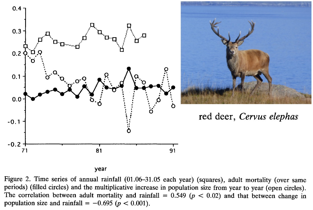 ] --- .large.pull-left-60[ ## If things are TOO random that spells trouble! According to theory, if: .darkred[$$\sigma_r > 2\mu_r$$] extinction is nearly certain - even if `\(\mu_r\)` is positive and on average there is growth. > .center[Experiment here: https://egurarie.shinyapps.io/StochasticGrowth] ] .pull-right-40[ ] --- ## some references - Benton, T. G., A. Grant, and T. H. Clutton-Brock. 1995. Does environmental stochasticity matter? Analysis of red deer life-histories on Rum. Evolutionary Ecology 9:559–574. - Estes, J. F. Palmisano. 1974. Sea otters: Their role in structuring nearshore communities. Science 185, 1058–1060. - Loshbaugh S. 2021. Sea Otters and the Maritime Fur Trade. In: Davis R.W., Pagano A.M. (eds) *Ethology and Behavioral Ecology of Sea Otters and Polar Bears. Ethology and Behavioral Ecology of Marine Mammals.* - Gilkinson, A.K., Pearson, H.C., Weltz, F. and Davis, R.W., 2007. Photo‐identification of sea otters using nose scars. *The Journal of Wildlife Management*, 71(6), pp.2045-2051. - Veltre, D.W. “Unangax̂: Coastal People of Far Southwestern Alaska”