Population Ecology III: Some Of All The Rest

class: center, top, title-slide

.title[
# Population Ecology III: Some Of All The Rest
]
.subtitle[
## .white[EFB 390: Wildlife Ecology and Management]
]
.author[
### Dr. Elie Gurarie
]
.date[
### October 29, 2024
]

---

## So far ...

We've studied this equation: `$\huge N_t = N_{t-1} + B_t - D_t$`

with two assumptions:

.pull-left.darkblue[

### Exponential Growth
**Births** and **Deaths** __proportional__ to **N**
]

.pull-right.darkgreen[
### Logistic Growth

**Births** decrease and/or **Deaths** decrease (.green[linearly?]) with **N**
]

---

## More complex topics in population ecology

Blowing up:

`$$\huge N_t$$`

**into:**

| | |
|---|----|
| sex / age classes: | **structured populations** |
| multiple sub-populations: |  **meta-populations** |
| multiple species: | **competitors / predator-prey** |
| infected, susceptible, recovered: | **disease dynamics** |

---

## Drilling into structure of Birth and Death

.blue[
`$$\Large N_t = N_{t-1} + B_t - D_t$$`
]

.box-blue[
.pull-left[
.large[**B** = Births]

- **Fecundity** = `#` births / female / unit time

(*unit time*  can be any unit of time, but is usually year)
]

.pull-right[

.large[**D** = Deaths]

- **Mortality (rate)** = probability of death / unit time

- **Survival (rate)** = 1 - Mortality rate
]
]

---

.pull-left-60[
## **Basic fact of life I:** Survival varies with age!

![](images/SSL_survival.png)
- **Survival Probability** ( `$S_0, S_1, S_2, ...$` ) always between 0 and 1.

- **Cumulative Survival** ( `$1, S_0, S_0 S_1, S_0 S_1 S_2, ...$` ) always starts at 1 and goes to 0

.center[([Altukhov et al. 2015](https://journals.plos.org/plosone/article?id=10.1371/journal.pone.0127292)
)]
]

.pull-right-40[

![](images/SSL_bully.jpg)
![](images/SSL_sleeping.jpg)

![](images/altukhov.png)

]

---

## **Basic fact of life II:** Fecundity varies with age!

![](images/ElephantFecundity.png)

.center[([Lahdenperä et al. 2015](https://frontiersinzoology.biomedcentral.com/articles/10.1186/s12983-014-0054-0))]

---
background-image: url("images/KhanLifeHistory.png")
background-size: cover
class:white

## .white[**Life History** is the reproduction / mortality pattern]

---

## Survival curves

.pull-left-60[
![](images/CurveTypes.png)
]

.pull-right-40.large[

- **TYPE I:** high survivorship for juveniles; most mortality late in life

- **TYPE II:** survivorship (or mortality) is relatively constant throughout life

- **TYPE III:** low survivorship for juveniles; survivorship high once older ages are reached
]

---

# Life history strategies: *r*-selected, vs. *K*-selected species

For a long time a popular **paradigm** (conceptual model purporting to explain a wide range of phenomenon) for understanding evolutionary drivers of life-history variation.   Still popularly taught:

.center[
![](images/rK-bunk.jpeg)
]

---
background-image: url("images/walrusoysters.png")
background-position: center
background-size: contain

.pull-left-30[
### r-selected species

#### strategy:

- lots of offspring
- little or no parental investment
- semelparous
- early maturity
- Type III survivorship 
- low survivorship
- short life-expectancy

#### drivers: 
- small size
- unstable / unpredictable environments

#### consequence
- highly fluctuating populations
]

.pull-right-30[

### K-selected species

#### strategy:

- few offspring
- lots of parental investment
- high survivorship
- late maturity
- iteroparous
- long life-expectancy
- Type I survivorship schedule

#### drivers:
- stable environments
- large

#### consequence
- more stable / slowly-fluctuating  populations

]

---

## Nice theory you've got there, but lots of counter-examples

.pull-left[
- What about **trees**?  They're big, they're long-lived (very **K**), but they produce and disperse a **heckload** of seeds (very, very **r**).
]

.pull-right[
- What about **iteroparous** species (**K**) that are hedging their bets against high inter-annual variation in environmental conditions (very **r**)? 
]

> .green[The r- and K-selection paradigm 
was  focussed on **density-dependent selection**. This paradigm 
was challenged as it became clear that ... **age-specific mortality** 
provide[s] a more mechanistic link between an environment and an 
**optimal life history** ...] ([Reznick et al. (2002) Ecology](https://esajournals.onlinelibrary.wiley.com/doi/full/10.1890/0012-9658%282002%29083%5B1509%3ARAKSRT%5D2.0.CO%3B2))

---
background-image: url("images/salmonids.png")
background-size: cover

## Salmonid (counter)-example

.center.large[

**Semelparous species**

Much bigger eggs (189 > 86 mg).

Also nest building and guarding behavior, before dying,

i.e. greater investment in **Juvenile Survival** over **Adult Survival**.

The iteros just keep staying alive and trying to

breed again and again. 
]
--

.pull-left.center[
> Inconsistent with **r**-**K** paradigm!
]

---

.pull-left[
### Tasmanian devil (*Sarcophilus harrisii*)

.center[<img src='images/tazzy.jpg' width='70%'/>]

Only marsupial carnivore | range restricted to Tasmania

.pull-left[
.darkred[Dying of *facial tumor disease*;  an infectious cancer (!) which kills nearly all adults > 3 years
]]

.pull-right[![](images/taztumor.jpeg)]
]

.pull-right-40[
### Switch to Semelparity

.green[**Previously:**  Longer-lived, and iteroparous, with later birth (over 1 year old)]

![](images/tazdevil_lifehistory.jpeg)

.darkblue[**Now:** Semelparous, one-shot, younger mothers (almost NO 2-3 year old animals!)] ([Jones et al. (2013)](https://doi.org/10.1073/pnas.0711236105))
]

---

##  *Monoceros academicus*: Three Life Stages

. | Larva | Sophomore | Emeritus |
--- |:----------:|:------:|:---:|
. | <img src='images/unicornlarva.webp' height='150px'/> | <img src='images/unicornstudent.jpg' height='150px'/> | <img src='images/oldunicorn.webp' height='150px%'/> |
 Survival | 0.5 |1 | 0 |
 Fecundity | 0 | 1.5 | 0.5 |
||||

> - **Survival** is a **probability** (unitless)
>
> - **Fecundity** is an **expected number** of offspring (n. ind.).

</center>

**Human experiment:**  8 volunteers please.

---

.pull-left-40[
## Experiment: results

Stage | Survival | Fecundity
----------|------|---
1. larvae  | 0.5  | 0
2. sophomore | 1    | 1
3. emeritus   | 0    | .5

See numerical experiment: https://egurarie.shinyapps.io/AgeStructuredGrowth/

]

.pull-right-60[
<img src="Lecture_PopulationEcology_PartIII_files/figure-html/runPop1-1.png" width="100%" />

]

>- Overall growth: `$\huge \lambda = 1$`

>- Stable age distribution: 50%, 25%, 25%

---

.pull-left-40[
## Change one value ....

Stage | Survival | Fecundity
----------|------|---
1. larvae | 0.5 | 0
2. sophomore | 1 | **2** 
3. emeritus | 0 | .5
]

.pull-right-60[
<img src="Lecture_PopulationEcology_PartIII_files/figure-html/runPop2-1.png" width="100%" />

>- Overall growth: `$\huge \lambda = 1.11$`

>- Stable distribution: 54%, 24% 22%

]

---

## *Monoceros academicus*: Type I

.pull-left[
<img src="Lecture_PopulationEcology_PartIII_files/figure-html/MonocerusTypeI-1.png" width="100%" />
]

.pull-right[

- **TYPE I:** high survivorship for juveniles; most mortality late in life.  Investment in young and survival.  Typical of long-lived species.

Stage | Survival | Fecundity
----------|------|---
1. larvae  | 0.5  | 0
2. sophomore | 1    | 1.5
3. emeritus   | 0    | .5
]

---

.pull-left-70[

## Pink Salmon (*Onchorrhynchus gorbusha*)

.pull-left[![](images/gorbusha.png)]
.pull-right[![](images/gorbusha-lifehistory.jpg)]
]

.pull-right-30[
### Strict 2-year life cycle

Year 0: 
- Spawn in late-summer 
- Hatch in winter
- Emerge in spring

Year 1: 
- Ocean phase

Year 2. 
- Enter freshwater late spring
- Spawn
- Die

]

---

## Pink Salmon (*Onchorrhynchus gorbusha*): Type III

.pull-left[
<img src="Lecture_PopulationEcology_PartIII_files/figure-html/OnchorhynchusTypeII-1.png" width="100%" />
]

.pull-right[

- **TYPE III:** low survivorship for juveniles; survivorship high once older ages are reached.  Basically - produce a whole boatload of offspring and hope for the best. Typically short-lived species.

Stage | Survival  | Fecundity
----------|-------|---
1. smolt  | 0.05   | 0
2. ocean  | 0.9   | 0
3. return | 0     | 21
]

---

# Life History Tables

>.large[Widely used classic tool to obtain life-history / survivorship curves ]

A "schedule" of all births and deaths in our population
- .darkblue[**Fecundity schedule:**] *how many* offspring are born by **age**

- .darkred[**Survivorship schedule:**] *with what probability* individuals by **age**

With those (& some tedious calculations) you can compute:

- **Life expectancy**

- Population **growth rate** `$\lambda$`

- **Age structure:**   .green[Are there lots of: young individuals? Old individuals? Reproductive age individuals?]

- **Survivorship patterns:** .green[Does most mortality occur in young / old / across ages?]

---
class: inverse

# Life History Tables - some "encouragement"

.center[![](images/gotelliencouragement.png)]

---
.pull-left-40[## Dall's sheep

Estimated life expectance: **7.2 years** 
But it if attains 6 years of age, anover **3.4 years**
]
.pull-right-60[.center[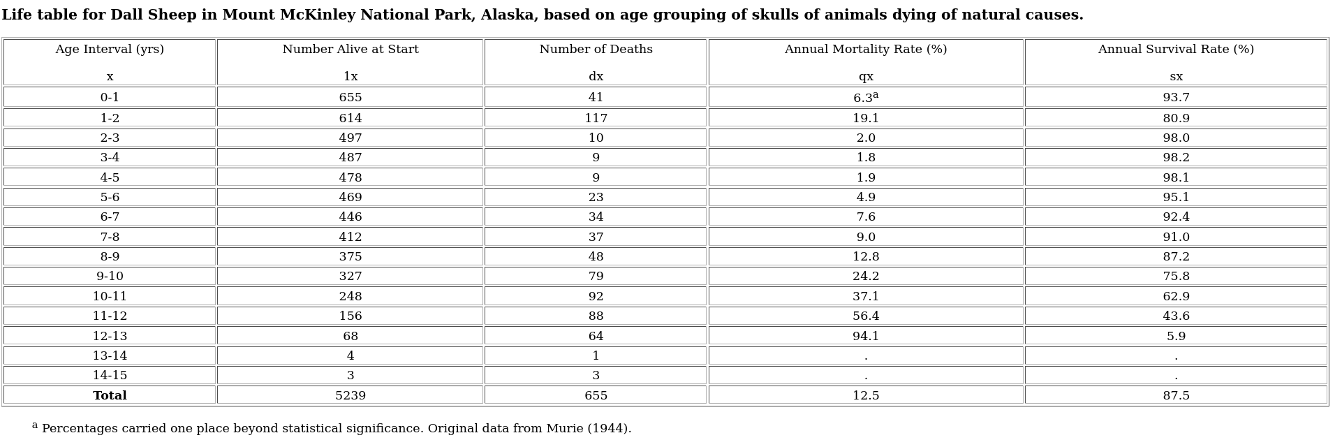![](images/dallssheep.png)]]

![](images/sheeplifetable.png)
.center[(from Murie 1944)]

---

## Estimating Life Histories: **Vertical Life Table**

.large[Take a snapshot of the age distribution and build survival schedule]

.pull-left-40[

.large[
**Strong assumptions:**

- `$r = 0$` or `$\lambda = 1$`

- processes (birth and survival schedules) are **stationary**, meaning .green[*parameters* don't change over time.]

- Of course - you also need to know **birth schedule**. 
]
]

.pull-right-60[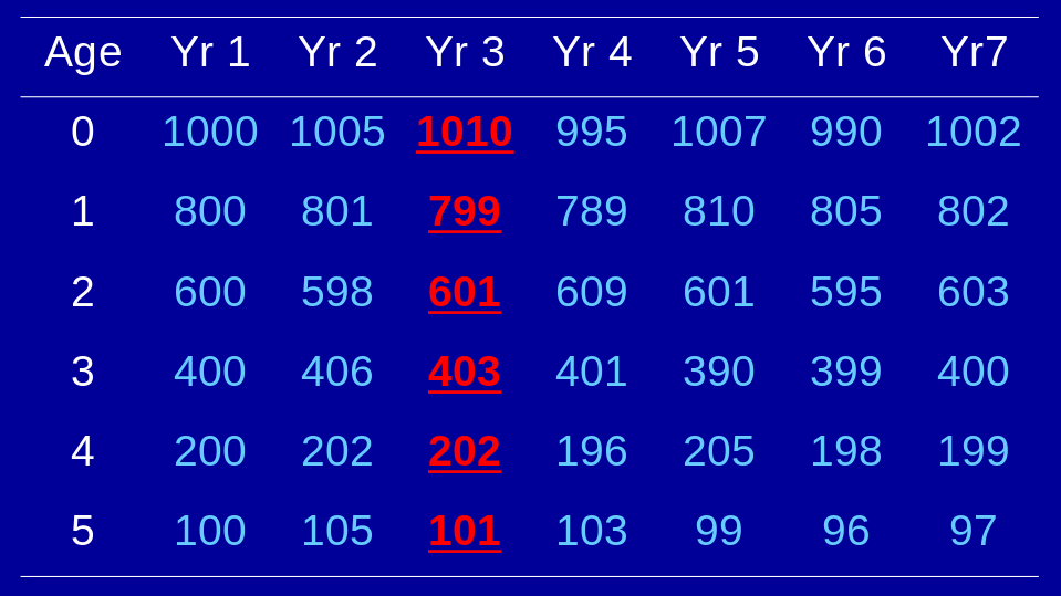

![](images/vertical.png)
]

---

## Estimating Life Histories: **Cohort Life Table**

.large[Follow a cohort (or cohorts) through time.  Track **survival**. Track **age at birth**.]

.pull-left-40[

.large[

**Minus:**

- Can take a really long time!

**Plus:**

- Population always decreasing!
]]

.pull-right-60[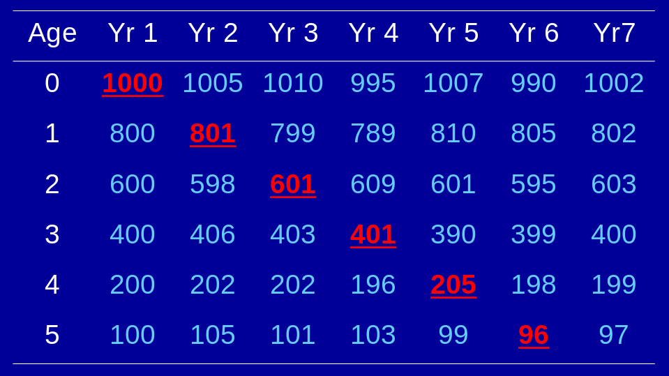
![](images/horizontal.png)
]

---
class:inverse

# Species Interactions

## Can also limit population growth

.pull-left-40.large[

- Competition

- Coexistence

- Predation

]

.pull-right-60[
![](images/elephantdog.jpg)]

---
class:inverse

#  Competition

.pull-left[
An interaction between organisms (intraspecific) or between species (interspecific) in which fitness of one is lowered by the presence of another.

*We've already talked about* ***intra***-*specific competition!*

### Fitness is Reproductive Success

- Combines **survival** and **reproduction**

]

.pull-right[
![](https://upload.wikimedia.org/wikipedia/commons/7/7f/Panthera_leo_%26_Crocuta_crocuta.jpg)
]

---

## Competitive Exclusion Principle

Two species **occupying the same niche** can NOT coexist

.pull-left[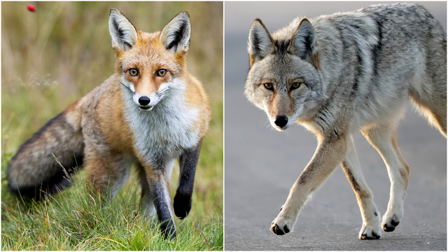![](images/foxandcoyote.jpg)

In *theory* Fox (*Vulpes vulpes*) and Coyote (*Canis latrans*) can't co-exist across southern Minnesota prairie / farmland
]

.pull-right[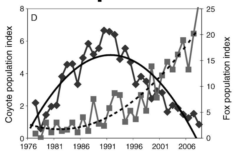
![](images/FoxCoyoteExclusion.png)

]

.center[[Levi and Wilmers (2021) *Ecology* 93(4)](https://doi.org/10.1890/11-0165.1)]

---

## Except they often do!  (via niche partitioning)

.pull-left[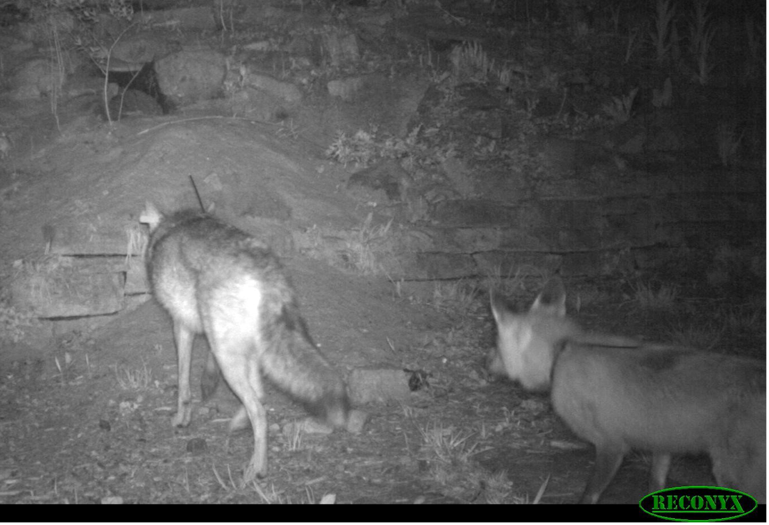![](images/FoxAndCoyote.png)

![](images/Mueller.png)
]
.pull-right-50[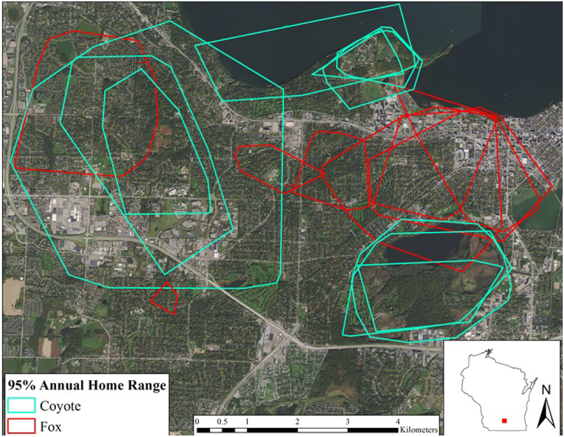
![](images/FoxCoyoteInMadison.png)

Madison, Wisconsin

]

---

## Squirlicorn vs. Pegamunk

Limited space | Limited carrying capacity |  Mutual animosity (periodic horn skewering and/or dropping on rocks) ....

.center[***Can they get along!?***

![](images/squirlicornvspegamunk_small.png)

https://egurarie.shinyapps.io/SquirlicornVsPegamunk
]

**Takeaway:**  If the interactions are not *too* extreme relative to population growth rate, coexistence is possible.

---

## Apparent competition

.large[Species A eats Species B and C, if Species B increases, Species C is in trouble.]

.pull-left-60[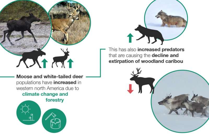![](images/apparent.jpg)]

.pull-right-40[
Major habitat fragmentation from oil-gas extraction.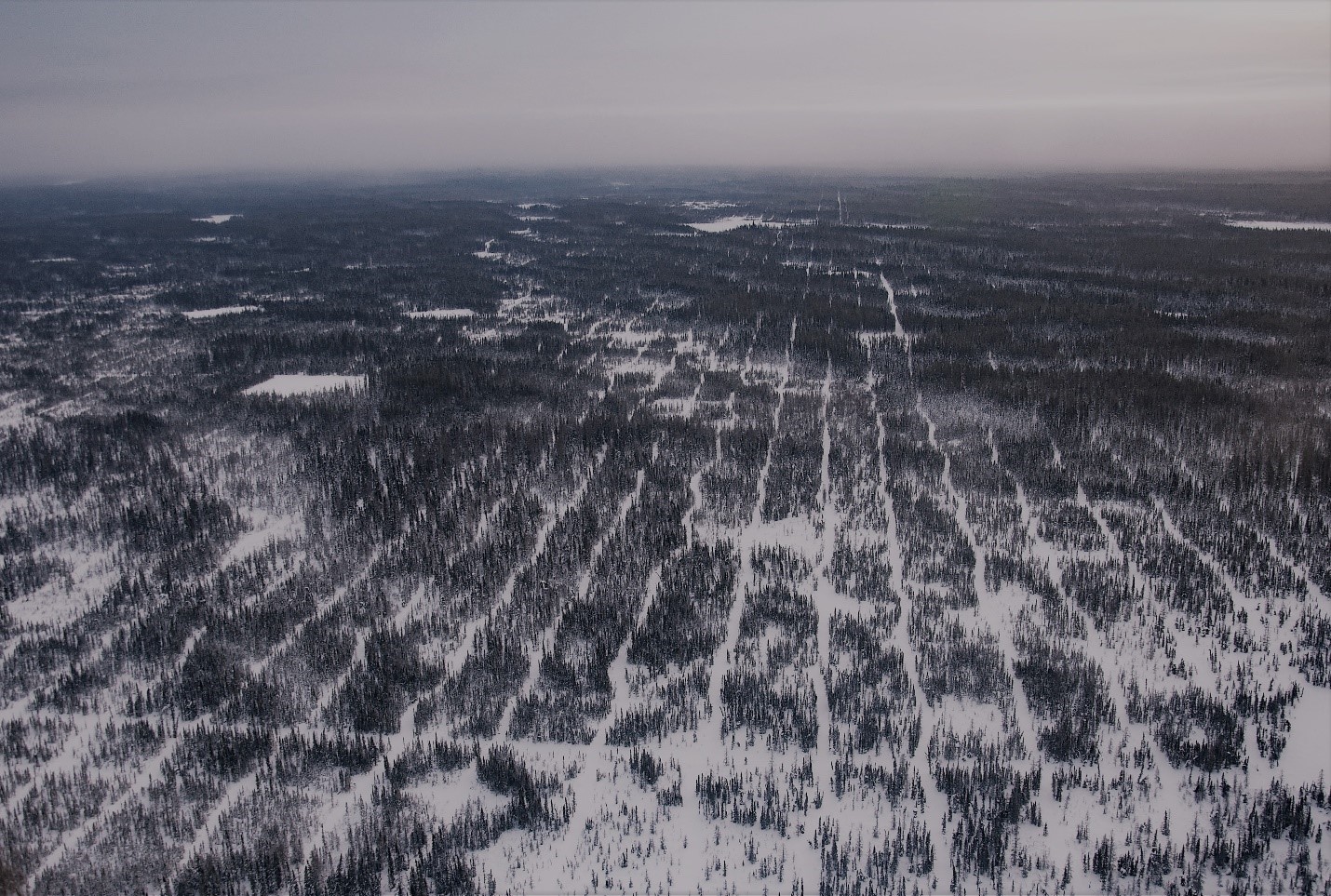

![](images/seismic.jpg)
***Serrouya et al. (2017)***
]

---
class: inverse

## Predation

.pull-left[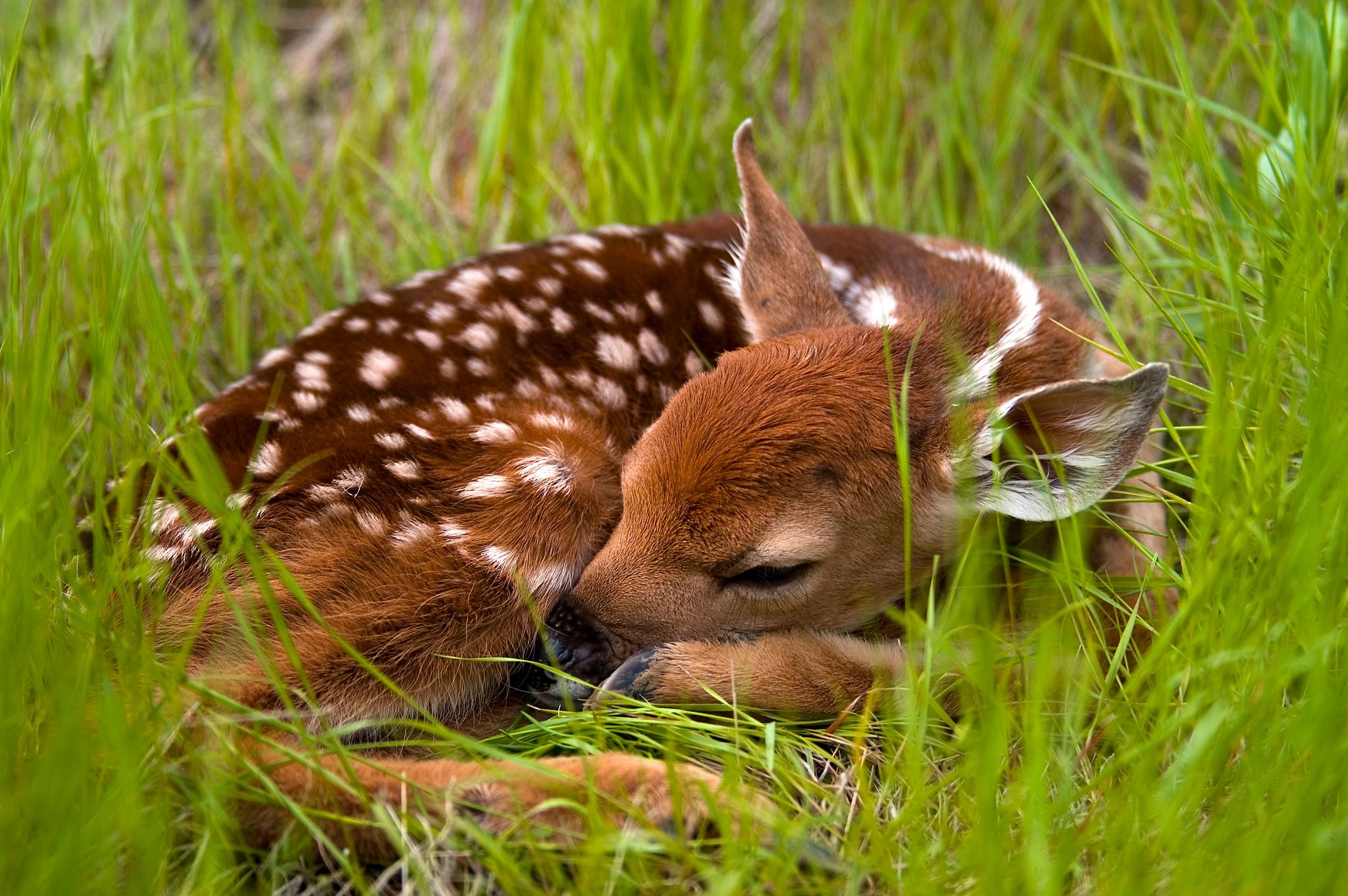
![](images/fawn.jpg)
]

.pull-right.large[

an ecological process where one organism (the predator) consumes another (the prey).

- Provides most of the principle route of energy flow through ecosystems

- Strong selective pressure

- **Chief source of density dependent effects** in regulation of many animal (and plant) populations
]

---

## Predator-prey dynamics

Based (mainly) on fur sales from the Hudson Bay Company in Canada over 100 years. Roughly a 9 to 11 year, fairly synchronous, cycle.

.pull-left-60[![](images/hare_lynx.png)]

.pull-right-40[![](images/harelynx_capture.jpg)]

.pull-wide[
Theory suggests the **predators** and **prey** cycle ... but it turns out that is *probably* not the case.]

---

## Equations and models

### Exponential model

.pull-left-40[
.red[
`$\large \frac{dN}{dt} = r N$`
]

Basic assumption: Growth rate is proportional to population size
]

.pull-right-60[![](examples/Exponential.png)]

---

## Equations and models

.pull-left[

### Exponential model

`$\large \frac{dN}{dt} = r N$`

.red[
### Logistic model

`$\large \frac{dN}{dt} = r N \left(1 - \frac{N}{K}\right)$`
]

Assumption growth rate goes to 0 at `$N=K$`

]

.pull-right-50[![](examples/Logistic.png)]

---

## Competition model

.pull-left[

.red[
`$${dC \over dt} = r_c C\left(1- {C\over K_c} - \alpha {F \over K_c}\right)$$`
`$${dF \over dt} = r_f F\left(1- {F \over K_f} - \beta {C \over K_f}\right)$$`
]
contains carrying capacities AND interactions
]

.pull-right-50[![](examples/Competition.png)]

---

## Predator-Prey Model

.pull-left-30[

.darkred[
`$\large {dP \over dt}  = -q P + \gamma VP$`
]
.blue[
`$\large {dV \over dt}  = r V - \sigma VP$`
]

]

.pull-right-70[![](examples/Predation.png)]

---
## Predator-Prey-Prey Model

.pull-left-30[

Wolf equation `$W(t)$`:
$${dW \over dt} = (\gamma_m M + \gamma_c C - \delta)W $$

Moose equation `$M(t)$`:
$${dM \over dt} = r_m M \left(1 - {M\over K_m}\right)  - \sigma_m MW $$

Woodland caribou equation `$C(t)$`:
$${dC \over dt} = r_c C \left(1 - {C\over K_c} \right)- \sigma_c CW $$
]

.pull-right-60[
![](images/ThreeBodyProblem.png)
]

---

## **To learn more:**

![](images/EFB370.png)

]

---

### Take-aways ....

.pull-left[
### Top-down

Sometimes predation is extremely important at limiting growth of prey populations.

![](images/top-down.png)
]

.pull-right[
### Bottom-up

Sometimes, predators are very much limited by the resources coming up the chain.

.pull-right-60[![](images/bottom-up.png)]
]

.large[ Resolving these questions is hard! (and interesting), and involves a combination of deep ecological research and modeling.]