class: center, top, title-slide .title[ # <strong>Population Ecology III: Structured Populations</strong> ] .subtitle[ ## .white[EFB 390: Wildlife Ecology and Management] ] .author[ ### <strong>Dr. Elie Gurarie</strong> ] .date[ ### October 30, 2025 ] --- <!-- https://bookdown.org/yihui/rmarkdown/xaringan-format.html --> ## So far ... We've studied this equation: `\(\huge N_t = N_{t-1} + B_t - D_t\)` with two assumptions: .pull-left.darkblue[ ### Exponential Growth **Births** and **Deaths** __proportional__ to **N** ] .pull-right.darkgreen[ ### Logistic Growth **Births** decrease and/or **Deaths** decrease (.green[linearly?]) with **N** ] --- ## More complex topics in population ecology Blowing up: `$$\huge N_t$$` **into:** | | | |---|----| | sex / age classes: | **structured populations** | | multiple sub-populations: | **meta-populations** | | multiple species: | **competitors / predator-prey** | | infected, susceptible, recovered: | **disease dynamics** | --- ## Drilling into structure of Birth and Death .blue[ `$$\Large N_t = N_{t-1} + B_t - D_t$$` ] .box-blue[ .pull-left[ .large[**B** = Births] - **Fecundity** = `#` births / female / unit time (*unit time* can be any unit of time, but is usually year) ] .pull-right[ .large[**D** = Deaths] - **Mortality (rate)** = probability of death / unit time - **Survival (rate)** = 1 - Mortality rate ] ] --- .pull-left-60[ ## **Basic fact of life I:** Survival varies with age!  - **Survival Probability** ( `\(S_0, S_1, S_2, ...\)` ) always between 0 and 1. - **Cumulative Survival** ( `\(1, S_0, S_0 S_1, S_0 S_1 S_2, ...\)` ) always starts at 1 and goes to 0 .center[([Altukhov et al. 2015](https://journals.plos.org/plosone/article?id=10.1371/journal.pone.0127292) )] ] .pull-right-40[    ] --- ## **Basic fact of life II:** Fecundity varies with age!  .center[([Lahdenperä et al. 2015](https://frontiersinzoology.biomedcentral.com/articles/10.1186/s12983-014-0054-0))] --- background-image: url("images/KhanLifeHistory.png") background-size: cover class:white ## .white[**Life History** is the reproduction / mortality pattern] --- ## Survival curves .pull-left-60[  ] .pull-right-40.large[ - **TYPE I:** high survivorship for juveniles; most mortality late in life - **TYPE II:** survivorship (or mortality) is relatively constant throughout life - **TYPE III:** low survivorship for juveniles; survivorship high once older ages are reached ] --- # Life history strategies: *r*-selected, vs. *K*-selected species For a long time a popular **paradigm** (conceptual model purporting to explain a wide range of phenomenon) for understanding evolutionary drivers of life-history variation. Still popularly taught: .center[  ] --- background-image: url("images/walrusoysters.png") background-position: center background-size: contain .pull-left-30[ ### r-selected species #### strategy: - lots of offspring - little or no parental investment - semelparous - early maturity - Type III survivorship - low survivorship - short life-expectancy #### drivers: - small size - unstable / unpredictable environments #### consequence - highly fluctuating populations ] .pull-right-30[ ### K-selected species #### strategy: - few offspring - lots of parental investment - high survivorship - late maturity - iteroparous - long life-expectancy - Type I survivorship schedule #### drivers: - stable environments - large #### consequence - more stable / slowly-fluctuating populations ] --- ## Nice theory you've got there, but lots of counter-examples .pull-left[ - What about **trees**? They're big, they're long-lived (very **K**), but they produce and disperse a **heckload** of seeds (very, very **r**). ] .pull-right[ - What about **iteroparous** species (**K**) that are hedging their bets against high inter-annual variation in environmental conditions (very **r**)? ] > .green[The r- and K-selection paradigm was focussed on **density-dependent selection**. This paradigm was challenged as it became clear that ... **age-specific mortality** provide[s] a more mechanistic link between an environment and an **optimal life history** ...] ([Reznick et al. (2002) Ecology](https://esajournals.onlinelibrary.wiley.com/doi/full/10.1890/0012-9658%282002%29083%5B1509%3ARAKSRT%5D2.0.CO%3B2)) --- background-image: url("images/salmonids.png") background-size: cover ## Salmonid (counter)-example <br><br><br> .center.large[ **Semelparous species** Much bigger eggs (189 > 86 mg). Also nest building and guarding behavior, before dying, i.e. greater investment in **Juvenile Survival** over **Adult Survival**. The iteros just keep staying alive and trying to breed again and again. ] -- .pull-left.center[ > Inconsistent with **r**-**K** paradigm! ] --- .pull-left[ ### Tasmanian devil (*Sarcophilus harrisii*) .center[<img src='images/tazzy.jpg' width='70%'/>] Only marsupial carnivore | range restricted to Tasmania .pull-left[ .darkred[Dying of *facial tumor disease*; an infectious cancer (!) which kills nearly all adults > 3 years ]] .pull-right[] ] -- .pull-right-40[ ### Switch to Semelparity .green[**Previously:** Longer-lived, and iteroparous, with later birth (over 1 year old)]  .darkblue[**Now:** Semelparous, one-shot, younger mothers (almost NO 2-3 year old animals!)] ([Jones et al. (2013)](https://doi.org/10.1073/pnas.0711236105)) ] --- ## *Monoceros academicus*: Three Life Stages . | Larva | Sophomore | Emeritus | --- |:----------:|:------:|:---:| . | <img src='images/unicornlarva.webp' height='150px'/> | <img src='images/unicornstudent.jpg' height='150px'/> | <img src='images/oldunicorn.webp' height='150px%'/> | <font size = 5> Survival | <font size = 5> 0.5 |<font size = 5>1 | <font size = 5>0 | <font size = 5> Fecundity |<font size = 5> 0 | <font size = 5>1.5 | <font size = 5>0.5 | |||| > - **Survival** is a **probability** (unitless) > > - **Fecundity** is an **expected number** of offspring (n. ind.). </center> -- **Human experiment:** 8 volunteers please. --- .pull-left-40[ ## Experiment: results Stage | Survival | Fecundity ----------|------|--- 1. larvae | 0.5 | 0 2. sophomore | 1 | 1 3. emeritus | 0 | .5 See numerical experiment: https://egurarie.shinyapps.io/AgeStructuredGrowth/ ] .pull-right-60[ <img src="Lecture_PopulationEcology_PartIII_files/figure-html/runPop1-1.png" width="100%" /> ] >- Overall growth: `\(\huge \lambda = 1\)` >- Stable age distribution: 50%, 25%, 25% --- .pull-left-40[ ## Change one value .... Stage | Survival | Fecundity ----------|------|--- 1. larvae | 0.5 | 0 2. sophomore | 1 | <font size = 6, color = "red"> **2** </font> 3. emeritus | 0 | .5 ] .pull-right-60[ <img src="Lecture_PopulationEcology_PartIII_files/figure-html/runPop2-1.png" width="100%" /> >- Overall growth: `\(\huge \lambda = 1.11\)` >- Stable distribution: 54%, 24% 22% ] --- ## *Monoceros academicus*: Type I .pull-left[ <img src="Lecture_PopulationEcology_PartIII_files/figure-html/MonocerusTypeI-1.png" width="100%" /> ] .pull-right[ - **TYPE I:** high survivorship for juveniles; most mortality late in life. Investment in young and survival. Typical of long-lived species. Stage | Survival | Fecundity ----------|------|--- 1. larvae | 0.5 | 0 2. sophomore | 1 | 1.5 3. emeritus | 0 | .5 ] --- .pull-left-70[ ## Pink Salmon (*Onchorrhynchus gorbusha*) .pull-left[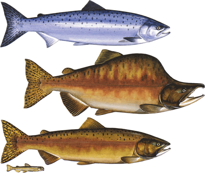] .pull-right[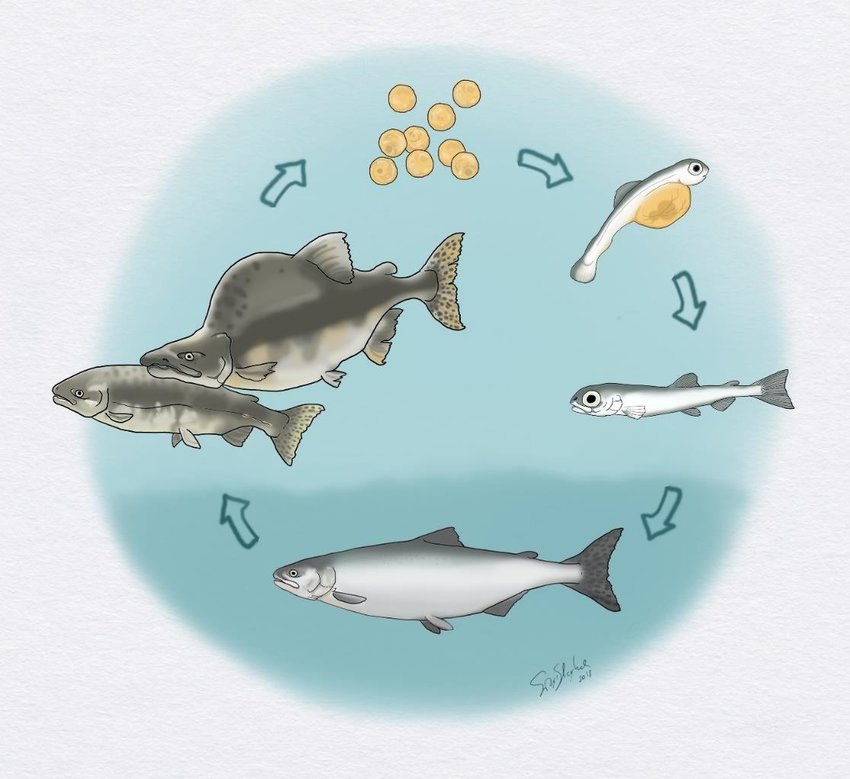] ] .pull-right-30[ ### Strict 2-year life cycle Year 0: - Spawn in late-summer - Hatch in winter - Emerge in spring Year 1: - Ocean phase Year 2. - Enter freshwater late spring - Spawn - Die ] --- ## Pink Salmon (*Onchorrhynchus gorbusha*): Type III .pull-left[ <img src="Lecture_PopulationEcology_PartIII_files/figure-html/OnchorhynchusTypeII-1.png" width="100%" /> ] .pull-right[ - **TYPE III:** low survivorship for juveniles; survivorship high once older ages are reached. Basically - produce a whole boatload of offspring and hope for the best. Typically short-lived species. Stage | Survival | Fecundity ----------|-------|--- 1. smolt | 0.05 | 0 2. ocean | 0.9 | 0 3. return | 0 | 21 ] --- # Matrix Models A **matrix** is a tool for **transforming vectors**. A **population matrix** transforms a structured population **vector** by 1. adding newborns, [fecundity: `\(f_i\)`] 2. killing off older classes, [survival: `\(s_i\)`] 3. scootching everyone up the stage ladder [aging] .pull-left[ `$$\begin{bmatrix} n_0 \\ n_1 \\ \vdots \\ n_{\omega - 1} \\ \end{bmatrix}_{t+1} = \begin{bmatrix} f_0 & f_1 & f_2 & \ldots & f_{\omega - 2} & f_{\omega - 1} \\ s_0 & 0 & 0 & \ldots & 0 & 0\\ 0 & s_1 & 0 & \ldots & 0 & 0\\ 0 & 0 & s_2 & \ldots & 0 & 0\\ \vdots & \vdots & \vdots & \ddots & \vdots & \vdots\\ 0 & 0 & 0 & \ldots & s_{\omega - 2} & 0 \end{bmatrix} \begin{bmatrix} n_0 \\ n_1 \\ \vdots\\ n_{\omega - 1} \end{bmatrix}_{t}$$` ] .pull-right-40[ **The Leslie Matrix** - is square - the rows and columns represent age classes - the top row is the number of **births** coming in from older age classes - the lower rows are the number of **survivors** into the next age class ] --- ## Remember *Monocerus academicus* ... .pull-left-60.center[ . | Larva | Sophomore | Emeritus | --- |:----------:|:------:|:---:| **Monoceros academicus** | <img src='images/unicornlarva.webp' height='100px'/> | <img src='images/unicornstudent.jpg' height='100px'/> | <img src='images/oldunicorn.webp' height='100px%'/> | Survival | 0.5 |1 | 0 | Fecundity | 0 | 1.5 | 0.5 | ] .pull-right-40[ Here's the matrix: $$ \large M = \\begin{bmatrix}0&1.5&0.5 \\\\0.5&0&0 \\\\0&1&0 \\\\\\end{bmatrix} $$ ] --- ## Leslie matrix as diagram The population matrix maps to a diagram! These are very useful: .pull-left-30[ ### Matrix $$ \Large M = \\begin{bmatrix}0&1.5&0.5 \\\\0.5&0&0 \\\\0&1&0 \\\\\\end{bmatrix} $$ ] .pull-right-70[ ### Diagram 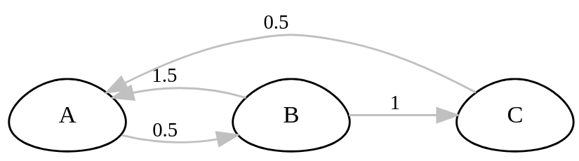 ] .box-grey[ - Arrow **A** to **B** (0.5) is represented by matrix entry **column 1** to **row 2** - survival to second stage. - Arrow **B** to **C** (1) is matrix entry **column 2** to **row 3** - survival to last stage. ] --- ## Amazing property of population matrices ... <br><br> `$$\huge M \times N^* = \lambda N^*$$` .large[ For every **population matrix** there is a **stable age distribution** for which the **population matrix** increases the **distribution vector** by a fixed proportion `\(\lambda\)`. - `\(\large N^*\)` - is "**eigenvector**" = .red[**stable population distribution**] - `\(\large \lambda\)` - is the "**eigenvalue**" = .red[**population growth factor**] ] --- ## *Monocerus academicus* .center[<img src='images/monodiagram.png' width = '50%' />] .pull-left[ ``` r matA <- rbind(c(0, 1.5, .5), c(.5, 0, 0), c(0, 1, 0)) ``` $$ \large M = \\begin{bmatrix}0&1.5&0.5 \\\\0.5&0&0 \\\\0&1&0 \\\\\\end{bmatrix} $$ ] .pull-right[ ``` r eigen(matA) ``` ``` ## eigen() decomposition ## $values ## [1] 1.0 -0.5 -0.5 ## ## $vectors ## [,1] [,2] [,3] ## [1,] -0.8164966 -0.4082483 0.4082483 ## [2,] -0.4082483 0.4082483 -0.4082483 ## [3,] -0.4082483 -0.8164966 0.8164966 ``` - First eigenvalue: `\(\lambda = 1\)` - Ratio of first eigenvector: 50% : 25% : 25% ] --- ## What if some emeriti decide to go back to school? <center> <img src='diag_backtoschool.png' width = '50%' /> </center> .pull-left-60[ $$ \large M = \\begin{bmatrix}0&1.5& 0.5 \\\\0.5&0&\color{red}{\textbf 0.5} \\\\0&1&0 \\\\\\end{bmatrix} $$ ] .pull-right-40[ ``` r eigen(matB) ``` ``` ## eigen() decomposition ## $values ## [1] 1.2071068 -1.0000000 -0.2071068 ## ## $vectors ## [,1] [,2] [,3] ## [1,] 0.7736915 0.5773503 0.6669930 ## [2,] 0.4878914 -0.5773503 0.1511012 ## [3,] 0.4041824 0.5773503 -0.7295812 ``` ] <br> <br> .large[ - First eigenvalue: `\(\lambda = 1.21\)` - Ratio of first eigenvector: 46% : 29% : 24% ] --- # Life History Tables >.large[Widely used classic tool to obtain life-history / survivorship curves ] A "schedule" of all births and deaths in our population - .darkblue[**Fecundity schedule:**] *how many* offspring are born by **age** - .darkred[**Survivorship schedule:**] *with what probability* individuals by **age** With those (& some tedious calculations) you can compute: - **Life expectancy** - Population **growth rate** `\(\lambda\)` - **Age structure:** .green[Are there lots of: young individuals? Old individuals? Reproductive age individuals?] - **Survivorship patterns:** .green[Does most mortality occur in young / old / across ages?] --- class: inverse # Life History Tables - some "encouragement" .center[] --- .pull-left-40[## Dall's sheep Estimated life expectance: **7.2 years** But it if attains 6 years of age, anover **3.4 years** ] .pull-right-60[.center[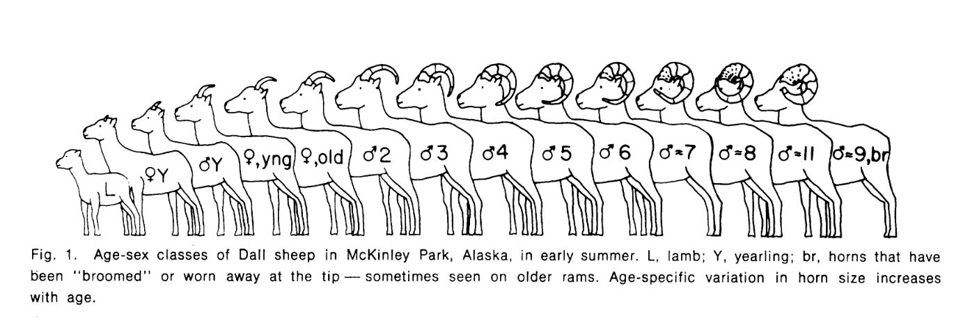]] 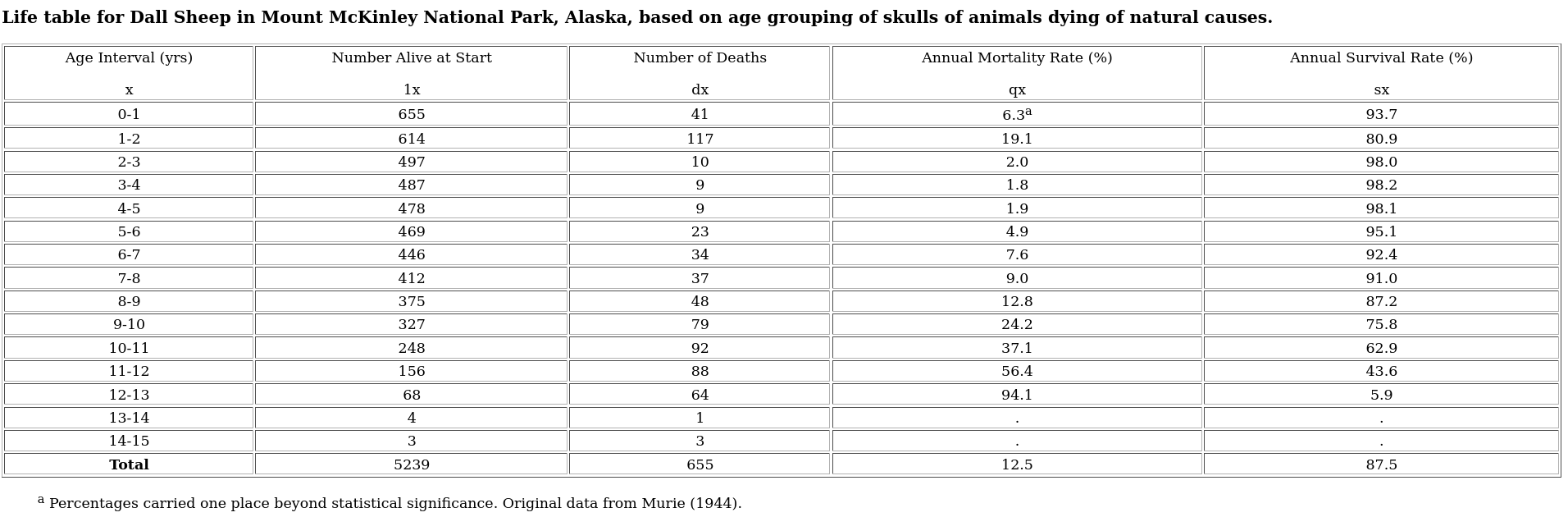 .center[(from Murie 1944)] --- ## Estimating Life Histories: **Vertical Life Table** .large[Take a snapshot of the age distribution and build survival schedule] .pull-left-40[ .large[ **Strong assumptions:** - `\(r = 0\)` or `\(\lambda = 1\)` - processes (birth and survival schedules) are **stationary**, meaning .green[*parameters* don't change over time.] - Of course - you also need to know **birth schedule**. ] ] .pull-right-60[  ] --- ## Estimating Life Histories: **Cohort Life Table** .large[Follow a cohort (or cohorts) through time. Track **survival**. Track **age at birth**.] .pull-left-40[ .large[ **Minus:** - Can take a really long time! **Plus:** - Population always decreasing! ]] .pull-right-60[  ] --- ## Do these assumptions hold? US population pyramid - 2020 .pull-left-70.pull-right-70[  ]