Loops and functions (and an animation

class: center, middle, inverse, title-slide

.title[
# Loops and functions (and an animation - for fun)
]
.subtitle[
## <a href="https://eligurarie.github.io/EFB654/">EFB 654: R and Reproducible Research</a>
]
.author[
### Elie Gurarie
]
.date[
### February 23, 2026
]

---

class: inverse

# Loops

---

## Simple `for` loop

``` r
for(i in 1:10)
  print(i)
```

```
## [1] 1
## [1] 2
## [1] 3
## [1] 4
## [1] 5
## [1] 6
## [1] 7
## [1] 8
## [1] 9
## [1] 10
```

`i` is the loop variable — it takes each value in the sequence, one at a time. 
- `i` is the most common name (**index**), but it's arbitrary.

---

## Pay attention to notation

``` r
names <- c("Aditya", "Bob", "Changzi", "Demetrious", "Ed")

# indexing style: i goes from 1 to the length of the vector
for(i in 1:length(names))
  print(nchar(names[i]))
```

```
## [1] 6
## [1] 3
## [1] 7
## [1] 10
## [1] 2
```

---

## Pre-allocate a container

Often you want to *save* results from a loop, not just print them. Make an empty container first, then fill it in.

``` r
nchars <- rep(NA, length(names))
for(i in 1:length(names))
 nchars[i] <- nchar(names[i])
nchars
```

```
## [1]  6  3  7 10  2
```

---

## Loop variable doesn't have to be an integer (or `i`)

``` r
for(n in names){
  print(n)
  print(nchar(n))
}
```

```
## [1] "Aditya"
## [1] 6
## [1] "Bob"
## [1] 3
## [1] "Changzi"
## [1] 7
## [1] "Demetrious"
## [1] 10
## [1] "Ed"
## [1] 2
```

---

## Saving results with element-based looping

Using a named vector:

``` r
nchars <- rep(NA, length(names))
names(nchars) <- names

for(n in names)
 nchars[n] <- nchar(n)
nchars
```

```
##     Aditya        Bob    Changzi Demetrious         Ed 
##          6          3          7         10          2
```

---

## Avoiding loops with `apply`

In R, loops can often be avoided with the `apply` family of functions:

``` r
sapply(names, nchar)
```

```
##     Aditya        Bob    Changzi Demetrious         Ed 
##          6          3          7         10          2
```

Also `plyr` / `dplyr` / tidyverse — we'll discuss this later.

> It is not very "R" to use a lot of loops!

---
class: inverse

# Uses of loops

---

## True iteration

Some problems genuinely require loops because each step depends on the previous one.

### Fibonacci sequence

``` r
fib <- rep(NA, 12)
fib[1] <- 1
fib[2] <- 1

for(i in 3:length(fib)){
 fib[i] <- fib[i-1] + fib[i-2]
}
fib
```

```
##  [1]   1   1   2   3   5   8  13  21  34  55  89 144
```

---

## Fibonacci in Nature

.pull-left[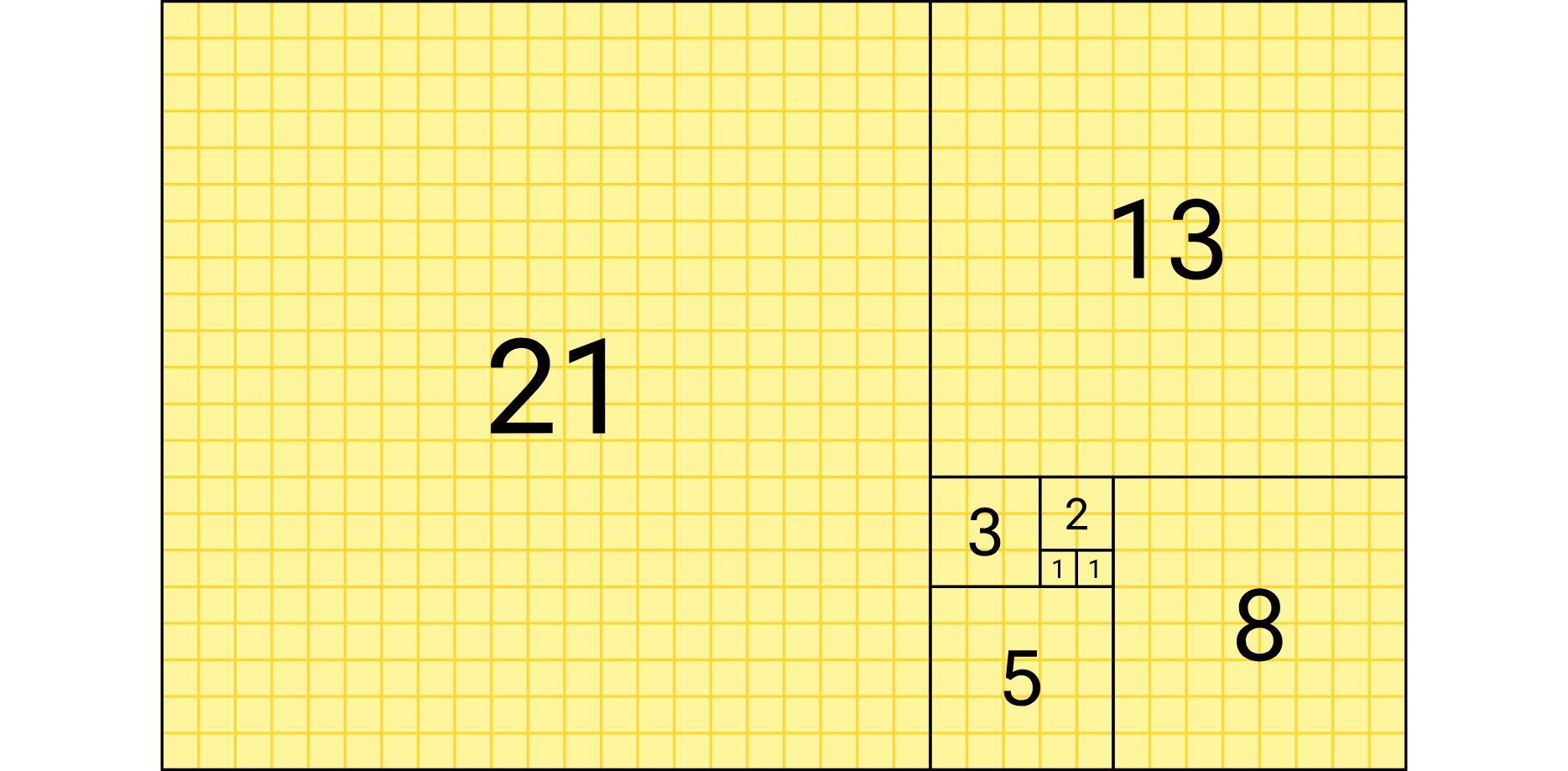
 
![](fibonacci1.png)

]

.pull-right[
![](fibonacci.webp)]

---

## A natural thing to wrap in a function
.pull-left[

``` r
computeFib <- function(n){
 fib <- rep(NA, n)
 fib[1] <- 1
 fib[2] <- 1
 
 for(i in 3:length(fib)){
 fib[i] <- fib[i-1] + fib[i-2]
 }
 fib
}
```
]

.pull-right[

``` r
(f30 <- computeFib(30))
```

```
##  [1]      1      1      2      3      5      8     13     21     34     55     89    144    233    377
## [15]    610    987   1597   2584   4181   6765  10946  17711  28657  46368  75025 121393 196418 317811
## [29] 514229 832040
```

``` r
f30[30]/f30[29]
```

```
## [1] 1.618034
```

Compare to golden ratio:  `$\large 1+\sqrt{5} \over 2$`

``` r
(1+sqrt(5))/2
```

```
## [1] 1.618034
```
]

---

.pull-left[
## Loop in loop

``` r
x <- seq(-5,5,.05)
y <- seq(-5,5,.05)

A <- matrix(NA, nrow = length(x), ncol = length(y))

for(i in 1:length(x))
 for(j in 1:length(y))
 A[i,j] <- cos(x[i]^2) * cos(y[j]^2)
```
]

.pull-right[

``` r
image(x,y,A, asp = 1)
```

]

---

## Looping through files

A very common real-world use: processing a batch of data files.

```
files <- list.files("path/to/csvs")
```

Example file listing from a CTT wildlife tracking project:

```
 [1] "CTT-V3033D437786-blu.2026-03-11_014627.csv"
 [2] "CTT-V3033D437786-blu.2026-03-11_024628.csv"
 [3] "CTT-V3033D437786-blu.2026-03-11_044631.csv"
 [4] "CTT-V3033D437786-blu.2026-03-11_164645.csv"
 [5] "CTT-V3033D437786-blu.2026-03-12_044659.csv"
 ...
```

``` r
for(f in files){
 mycsv <- read.csv(f)
 # do something with mycsv
}
```

---

## `while` loops

A `while` loop repeats as long as a condition is `TRUE`. The condition is checked *before* each iteration.  Example below runs the Fibonacci iteration up to a certain value:

``` r
fib <- c(1, 1)
while(fib[length(fib)] < 1000){
 fib <- c(fib, fib[length(fib)] + fib[length(fib)-1])
}
fib
```

```
##  [1]    1    1    2    3    5    8   13   21   34   55   89  144  233  377  610  987 1597
```

---

## Be careful!

.pull-left[

If the condition never becomes `FALSE`, the loop runs forever:

``` r
# Do NOT run this
x <- 2
while(x > 1){
 x <- x + 1
 cat(paste(x, " "))
}
```
]

.pull-right[

Often, you can put in an `if` statement and `stop` or `break` command to break a loop:

``` r
x<- 2
while(x > 1){
 x <- x + 1
 cat(paste(x, " "))
 if(x > 100) stop("woah!")
}
```

Though here - of course - it's easier to just put a roof: `while(x < 100)` 
]

---

## Example: finding the maximum of a function

``` r
funkycurve <- function(x) x^2 * sin(x) / (1 + x)
curve(funkycurve(x), xlim = c(0, 5), lwd = 2)
```

---

## Finding the max with a `while` loop

A simple `while` loop to find the max between 0 and 5 within a tolerance of 0.001:

.pull-left[

``` r
lo <- 0; hi <- 5; tol <- 0.001

while((hi - lo) > tol){
 mid <- (lo + hi) / 2
 if(funkycurve(mid + tol) > funkycurve(mid - tol)){
 lo <- mid
 } else {
 hi <- mid
 }
}
```
]

.pull-right[

``` r
mid
```

```
## [1] 2.125854
```

``` r
funkycurve(mid)
```

```
## [1] 1.228714
```
]

> Think through how this algorithm works....

---

## Visualize the result

``` r
curve(funkycurve(x), xlim = c(0, 5), lwd = 2)
abline(v = mid, lty = 2, col = "red", lwd = 2)
```

---

## Looping through years of WDI data

``` r
load("WDI_allyears.rda")
with(WDI, table(country))
```

---

## Define a plotting function

.small[

``` r
plotWDI <- function(myyear, ...){
 
 cols <- c("East Asia & Pacific" = "steelblue",
 "Europe & Central Asia" = "forestgreen",
 "Latin America & Caribbean" = "goldenrod",
 "Middle East & North Africa" = "darkorange",
 "North America" = "mediumpurple",
 "South Asia" = "firebrick",
 "Sub-Saharan Africa" = "sienna")
 
 mywdi <- subset(WDI, year == myyear)
 mywdi_big <- mywdi[order(mywdi$Population, decreasing = TRUE),][1:10,]
 
 cont_col <- cols[match(mywdi$region, levels(mywdi$region))]
 cex_pop <- sqrt(mywdi$Population / max(mywdi$Population, na.rm = TRUE)) * 15
 
 with(mywdi, {
 plot(GDP/1e3, LifeExp, log = "x",
 ylab = "Life expectancy (years)",
 xlab = "GDP per capita (1000 USD, log scale)", 
 type = "n", ...)
 grid()
 points(GDP/1e3, LifeExp,
 cex = cex_pop + .5, pch = 21, col = cont_col,
 bg = scales::alpha(cont_col, .7))
 legend("bottomright", title = "Region",
 legend = levels(region),
 pt.bg = cols, col = "grey40",
 pch = 21, pt.cex = 1.8, bty = "n", cex = 0.7)
 title(paste("Health v. Wealth", myyear))
 })
}
```
]

---
## Example of function use

.pull-left[

``` r
load("WDI_allyears.rda")
plotWDI(1960, xlim = c(.01, 2e2), ylim = c(25, 90))
```

<img src="loops_slides_files/figure-html/unnamed-chunk-25-1.png" alt="" style="display: block; margin: auto;" />
]

.pull-right[

``` r
plotWDI(2020,
        xlim = c(.01, 2e2), ylim = c(25, 90))
```

]

---

## Loop to create a multi-page PDF

``` r
pdf("HealthVWealth.pdf", width = 10, height = 8)
  par(mar = c(4,4,3,2),
      cex.axis = 0.8, family = "serif",  
      tck = 0.01, mgp = c(2,.25,0), las = 1)
  for(myy in 1960:2023)
    plotWDI(myy, 
            xlim = c(.01, 2e2),
            ylim = c(25, 90))
dev.off()
```

---

## Or loop to create many PNGs

``` r
for(myy in 1960:2023){
  png(paste0("pngs/healthvwealth", myy, ".png"), 
      width = 800, height = 600, res = 120)
    par(mar = c(4,4,3,2),
        cex.axis = 0.8, family = "serif",  
        tck = 0.01, mgp = c(2,.25,0), 
        las = 1)
      plotWDI(myy, 
              xlim = c(.01, 2e2),
              ylim = c(25, 90))
  dev.off()
}
```

---

## Animate with the `magick` package
.pull-left-40[

``` r
library(magick)
pngs <- list.files("pngs", pattern = "*.png", full.names = TRUE)
frames <- image_read(pngs)
anim <- image_animate(frames, fps = 5)
image_write(anim, "HealthVWealth.gif")
```
]

.pull-right-60[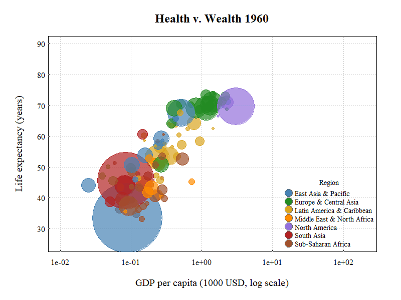
![](HealthVWealth.gif)
]