Linear Models with Spatial Correlations
EFB 796: Practical Seminar in Quantitative Ecology
Elie Gurarie
2025-03-19
2 The Linear Model
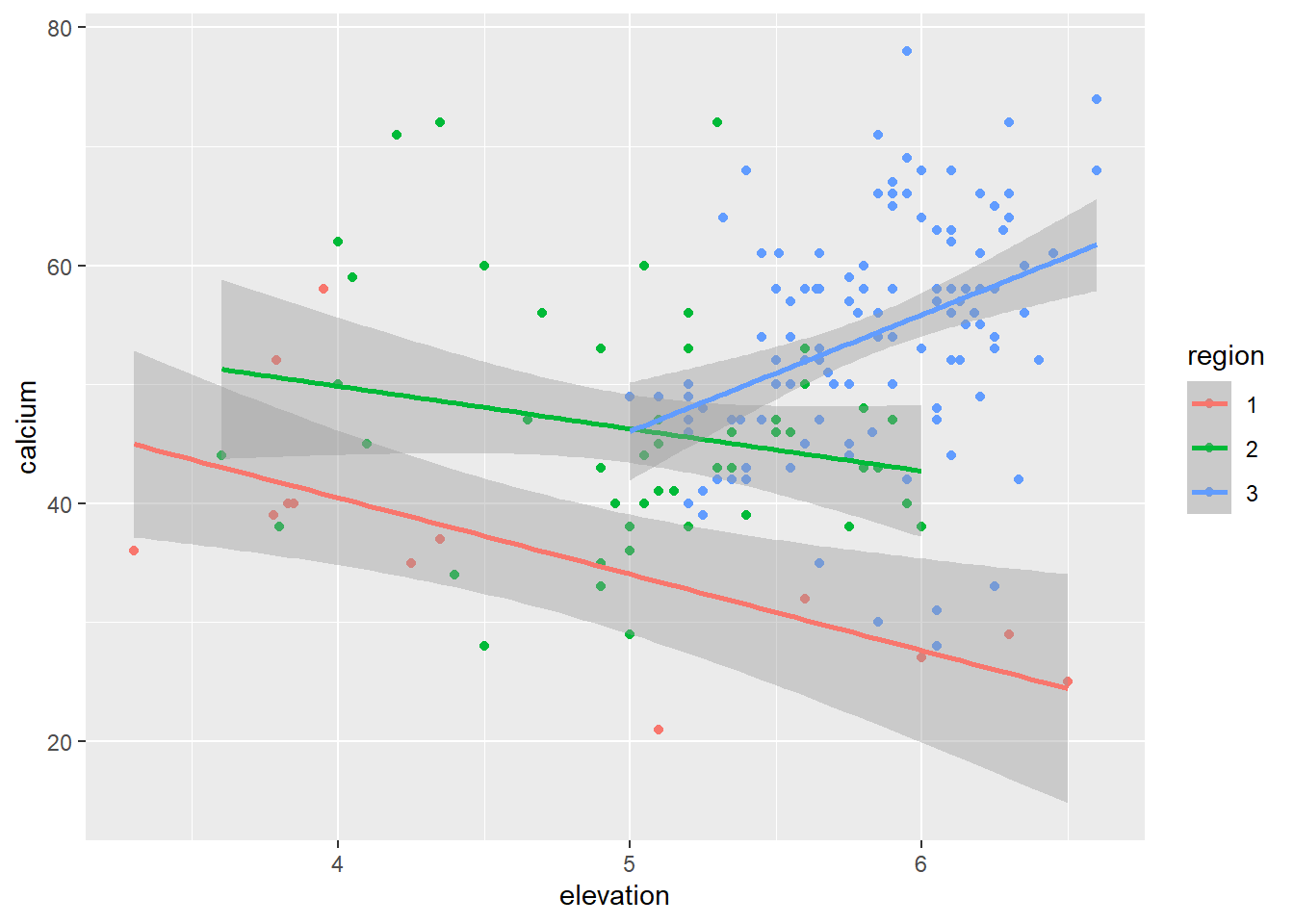
A linear model
Ca_lm <- lm(calcium ~ elevation * region, data = dat)
summary(Ca_lm)##
## Call:
## lm(formula = calcium ~ elevation * region, data = dat)
##
## Residuals:
## Min 1Q Median 3Q Max
## -28.3603 -5.0931 -0.4355 5.5786 26.7756
##
## Coefficients:
## Estimate Std. Error t value Pr(>|t|)
## (Intercept) 66.179 11.486 5.762 3.76e-08 ***
## elevation -6.425 2.403 -2.673 0.008235 **
## region2 -2.082 16.063 -0.130 0.897031
## region3 -69.182 17.980 -3.848 0.000168 ***
## elevation:region2 2.864 3.270 0.876 0.382361
## elevation:region3 16.237 3.374 4.812 3.25e-06 ***
## ---
## Signif. codes: 0 '***' 0.001 '**' 0.01 '*' 0.05 '.' 0.1 ' ' 1
##
## Residual standard error: 9.133 on 172 degrees of freedom
## Multiple R-squared: 0.3398, Adjusted R-squared: 0.3206
## F-statistic: 17.7 on 5 and 172 DF, p-value: 3.908e-14What are the main inferences?
2.1 Assessing residuals
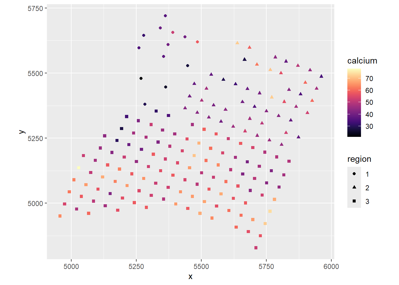
It’s residuals
dat$res <- Ca_lm$residualsggplot(dat, aes(x, y, color = res, shape = region)) +
geom_point() +
scale_color_viridis(option = "A") +
coord_fixed()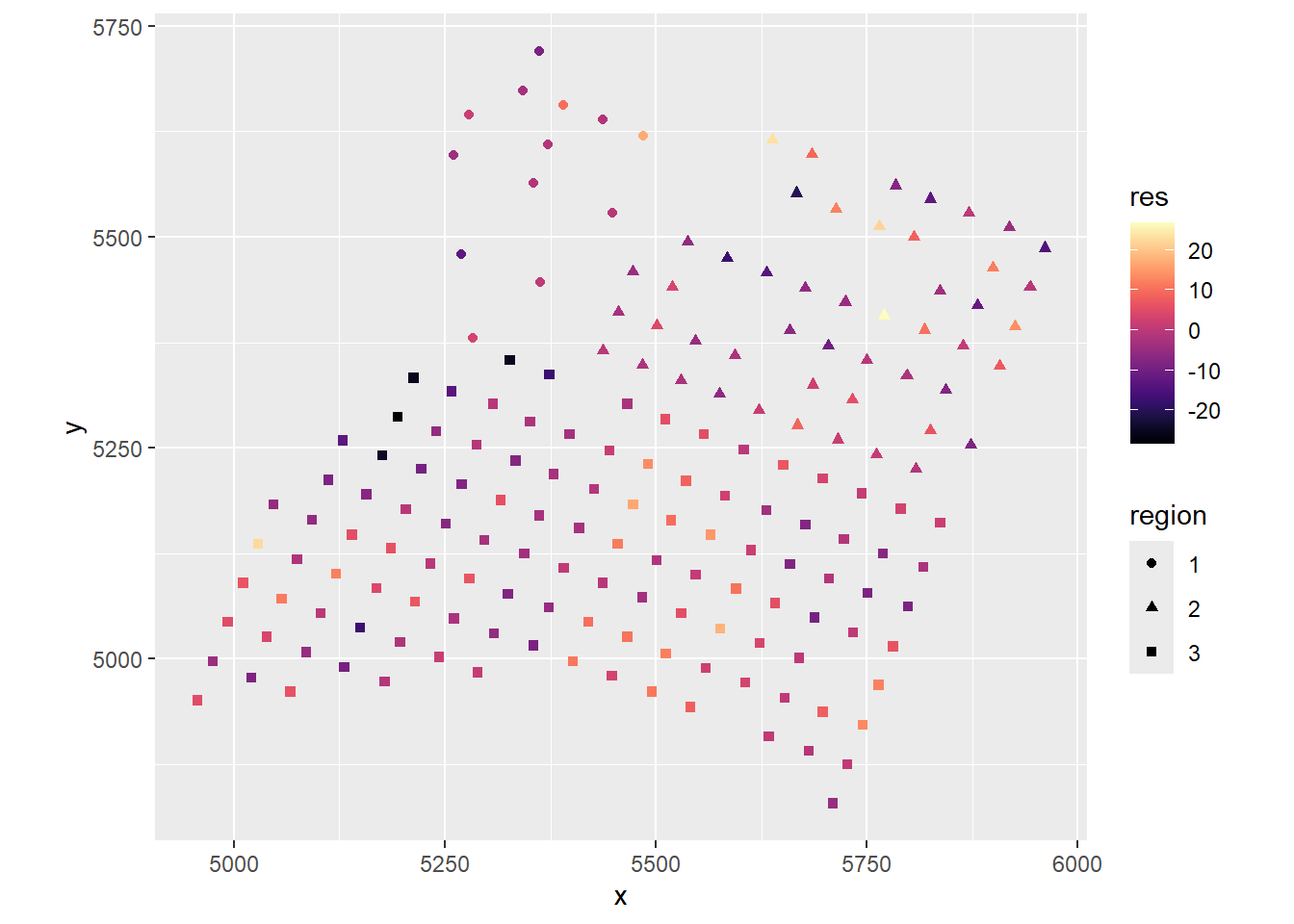 There is definitely spatial autocorrelation in the residuals!
2.2 Moran’s I test
If you want to obtain a statistical measure for spatial correlation, there is a Widely used statistic called Moran’s I.
2.3 Formula
\[ I = \frac{n}{s} \times \frac{\sum_{i} \sum_{j} w_{ij} (x_i - \bar{x}) (x_j - \bar{x})}{\sum_{i} (x_i - \bar{x})^2} \]
Where: - \(n\) = total number of observations - \(x_i, x_j\) = values at locations \(i\) and \(j\) - \(\bar{x}\) = mean of the variable - \(w_{ij}\) = spatial weight between locations \(i\) and \(j\) - \(s = \sum_{i} \sum_{j} w_{ij}\), the sum of all spatial weights
The weights between the locations represent a structural assumption about the nature of the relationship between points as a function of distance \(d_{ij}\). In practice, it is almost always of the from \(1/d_{ij}^p\), where \(p\) is either 1 or 2.
If \(I \approx 0\), there is no significant spatial autocorrelation. If the statistic is positive \(I > 0\), similar values cluster together, if it is negative (something I’ve never seen) dissimilar values are adjacent.
The ape::Moran.I() computes Moran’s I, but you have to
specify weights:
require(ape)
# compute distance metric
D.matrix <- dist(dat[,c("x","y")]) |> as.matrix()
w <- 1/D.matrix
# set diagonals to 0
diag(w) <- 0
Moran.I(dat$res, w)## $observed
## [1] 0.03825488
##
## $expected
## [1] -0.005649718
##
## $sd
## [1] 0.006872627
##
## $p.value
## [1] 1.677087e-10The inverse distance weights have a highly significant positive Moran’s I. Same for the squared distance:
Moran.I(dat$res, w^2)## $observed
## [1] 0.1205907
##
## $expected
## [1] -0.005649718
##
## $sd
## [1] 0.02000301
##
## $p.value
## [1] 2.77111e-10If you like prettier output (but less control) here’s a function in
the DHARMa package:
require(DHARMa)
testSpatialAutocorrelation(dat$res, dat$x, dat$y, plot=FALSE)##
## DHARMa Moran's I test for distance-based autocorrelation
##
## data: dat$res
## observed = 0.0382549, expected = -0.0056497, sd = 0.0068726, p-value =
## 1.677e-10
## alternative hypothesis: Distance-based autocorrelation3 Modeling with spatial correlation
Ok, we definitely have correlated residuals. We need to take those into account. So, our model might look like:
\[Y = X\beta + \epsilon\]
where
\[\epsilon \sim {\cal N}(0, \Sigma)\]
What distinguishes this from a standard ordinarily squares regression is that the residuals are not independent, but correlated. Our task is to find a reasonable correlation structure.
For example, for the above, we might assume a spatial Gaussian correlation structure in the residuals that assumes:
\[\Sigma_{ij} = \sigma^2 \, Cor(r_i,r_j) = \sigma^2 (1-\nu) \exp\left(-(d_{ij} / \delta)^2 \right)\]
Where \(d_{ij} = ||z_i - z_j||\) is the distance between the two residuals. There are now three parameters to estimate in the \(\Sigma\): the overall variance \(\sigma^2\), the “nugget” \(0 \leq \nu \leq 1\) and the distance scale \(\delta > 0\). The nugget captures the variation among points sampled int the same location (where \(\delta_{ij} = 0\)) - if it equal to 0 we assume all the observations at a given location is the same. The \(\delta\) is the distance parameter - it captures the spatial scale of autocorrelation.
3.1 Generalized least
squares (gls)
Generalized Least Squares is an efficient matrix-inversion based statistical method (as you might guess it generalizes the standard least squares approach with a fancier \(\Sigma\)) for estimating exactly this model. It is efficient and exact - unfortunately it only works on Gaussian models.
Here’s an example.
require(nlme)
Ca_gls_gauss <- gls(calcium ~ elevation * region,
correlation = corGaus(1, ~ I(x/100) + I(y/100), nugget = TRUE),
data = dat)
summary(Ca_gls_gauss)## Generalized least squares fit by REML
## Model: calcium ~ elevation * region
## Data: dat
## AIC BIC logLik
## 1250.789 1279.116 -616.3945
##
## Correlation Structure: Gaussian spatial correlation
## Formula: ~I(x/100) + I(y/100)
## Parameter estimate(s):
## range nugget
## 0.5568721 0.1761542
##
## Coefficients:
## Value Std.Error t-value p-value
## (Intercept) 55.28398 13.221775 4.181283 0.0000
## elevation -3.96324 2.613188 -1.516629 0.1312
## region2 5.10573 20.015049 0.255095 0.7990
## region3 -47.20941 22.935333 -2.058370 0.0411
## elevation:region2 1.06267 3.942516 0.269540 0.7878
## elevation:region3 11.84809 4.112586 2.880935 0.0045
##
## Correlation:
## (Intr) elevtn regin2 regin3 elvt:2
## elevation -0.972
## region2 -0.652 0.630
## region3 -0.565 0.545 0.352
## elevation:region2 0.634 -0.650 -0.983 -0.334
## elevation:region3 0.605 -0.619 -0.379 -0.986 0.383
##
## Standardized residuals:
## Min Q1 Med Q3 Max
## -2.95482414 -0.48688629 -0.03463241 0.60893645 2.87029479
##
## Residual standard error: 9.400885
## Degrees of freedom: 178 total; 172 residualNote, I had to divide the X in my coordinates by a 100 in order to make the algorithm work. Lots of good information here. Look at the results and answer The following questions:
- What is the spatial scale of correlation?
- What is an interpretation of the nugget estimate?
- Where in this output is an estimate of \(\sigma^2\)?
- Are the main effects results different than when we did not account for spatial correlation?
3.2 Exponential correlation
The exponential spatial correlation looks just like the Gaussian one, except it isn’t squared.
\[\Sigma_{ij} = \sigma^2 \, Cor(r_i,r_j) = \sigma^2 (1-\nu) \exp\left(-d_{ij} / \delta \right)\]
require(nlme)
Ca_gls_exp <- gls(calcium ~ elevation * region,
correlation = corExp(1, ~ I(x/100) + I(y/100), nugget = TRUE),
data = dat)
summary(Ca_gls_exp)## Generalized least squares fit by REML
## Model: calcium ~ elevation * region
## Data: dat
## AIC BIC logLik
## 1246.11 1274.437 -614.0549
##
## Correlation Structure: Exponential spatial correlation
## Formula: ~I(x/100) + I(y/100)
## Parameter estimate(s):
## range nugget
## 1.1725469 0.1585413
##
## Coefficients:
## Value Std.Error t-value p-value
## (Intercept) 53.32160 15.393860 3.463823 0.0007
## elevation -2.49907 2.779489 -0.899110 0.3699
## region2 -12.50173 23.528630 -0.531341 0.5959
## region3 -36.13745 25.569560 -1.413300 0.1594
## elevation:region2 3.48074 4.302498 0.809005 0.4196
## elevation:region3 8.71906 4.406387 1.978733 0.0494
##
## Correlation:
## (Intr) elevtn regin2 regin3 elvt:2
## elevation -0.943
## region2 -0.619 0.561
## region3 -0.601 0.579 0.371
## elevation:region2 0.574 -0.570 -0.973 -0.313
## elevation:region3 0.589 -0.624 -0.354 -0.978 0.332
##
## Standardized residuals:
## Min Q1 Med Q3 Max
## -2.48364728 -0.52071961 -0.02756801 0.55888847 2.49242099
##
## Residual standard error: 10.79667
## Degrees of freedom: 178 total; 172 residualNote how the range and nugget changed.
We can compare these two spatial correlation structures:
AIC(Ca_gls_exp, Ca_gls_gauss)## df AIC
## Ca_gls_exp 9 1246.110
## Ca_gls_gauss 9 1250.789There is some evidence that the exponential model is better one. But is there a better way to determine this? Or a more flexible spatial correlation structure?
Why yes! Is is the …..
3.3 Matérn correlation
A more generalized form of spatial autocorrelation is the Matérn covariance function. Before we get into it, here are the only pictures I could find of Bertil Matérn (1917-2007) - the Swedish forestry statistician for whom this covariance structure is named:
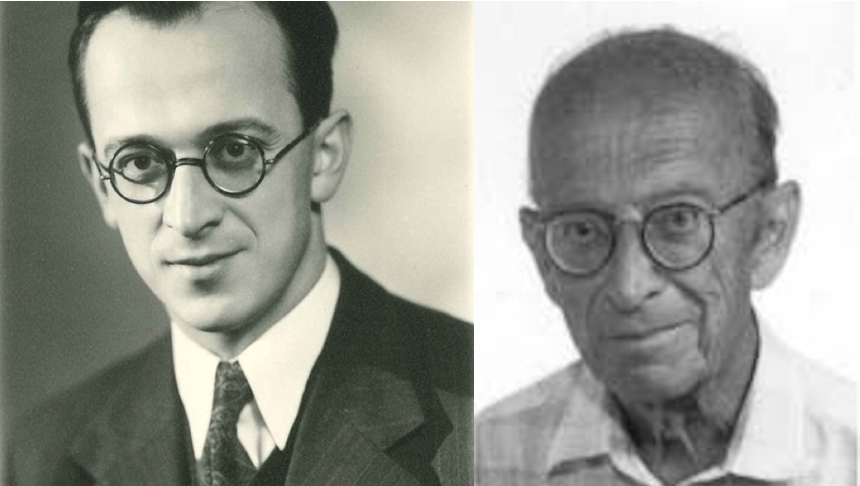
From these, we can infer that he never changed his expression or glasses style in 7 decades. However, he must have been relieved when the top of his head grew back, after being presumably blown away by this thing:
\[C_\nu(d) = \sigma^2\frac{2^{1-\nu}}{\Gamma(\nu)}\Bigg(\sqrt{2\nu}\frac{d}{\rho}\Bigg)^\nu K_\nu\Bigg(\sqrt{2\nu}\frac{d}{\rho}\Bigg)\]
This is the Matérn distance function. It’s not that important to know what \(\Gamma\), \(K\), etc. are (you can dig into it )
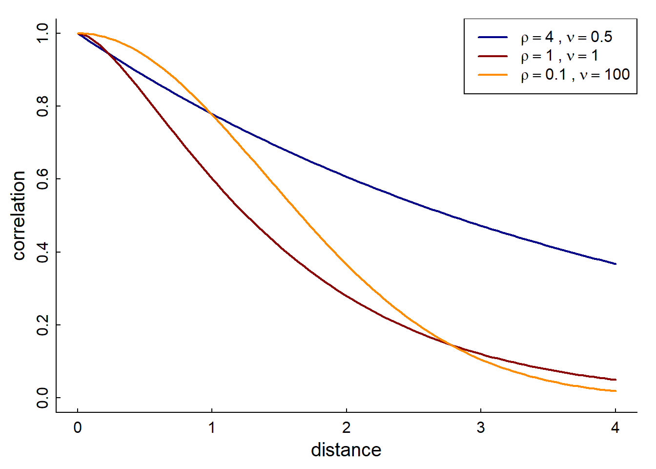
The parameter \(\mu\) is refered to
as “smoothness”, and \(\rho\) is the
“scale” (similar to \(\delta\) above).
At \(\nu = 1/2\) it is exponential. At
\(\nu \to \infty\) it is Gaussian. But
it is generally quite flexible. So if you don’t want to pre-specify that
shape, the Matern approach will allow you to estimate both those
parameters. Here’s an example using the spaMM package:
library(spaMM)
m_spamm <- fitme(calcium ~ elevation * region + Matern(1 | x + y),
data = dat, family = "gaussian")
# model summary
summary(m_spamm)## formula: calcium ~ elevation * region + Matern(1 | x + y)
## ML: Estimation of corrPars, lambda and phi by ML.
## Estimation of fixed effects by ML.
## Estimation of lambda and phi by 'outer' ML, maximizing logL.
## family: gaussian( link = identity )
## ------------ Fixed effects (beta) ------------
## Estimate Cond. SE t-value
## (Intercept) 52.561 13.718 3.8317
## elevation -2.937 2.613 -1.1242
## region2 -2.714 20.959 -0.1295
## region3 -38.370 23.703 -1.6188
## elevation:region2 2.145 3.993 0.5372
## elevation:region3 9.709 4.174 2.3262
## --------------- Random effects ---------------
## Family: gaussian( link = identity )
## --- Correlation parameters:
## 1.nu 1.rho
## 0.44908106 0.01530941
## --- Variance parameters ('lambda'):
## lambda = var(u) for u ~ Gaussian;
## x + y : 90.21
## # of obs: 178; # of groups: x + y, 178
## -------------- Residual variance ------------
## phi estimate was 0.00499297
## ------------- Likelihood values -------------
## logLik
## logL (p_v(h)): -626.335So - here we have estimates: \(\nu = 0.43\) and \(\rho = 0.0116\). What does that look like?
curve(MaternCorr(x, nu = 0.43, rho = 0.01), xlim = c(0,500))
abline(h = 0.1, lty = 3)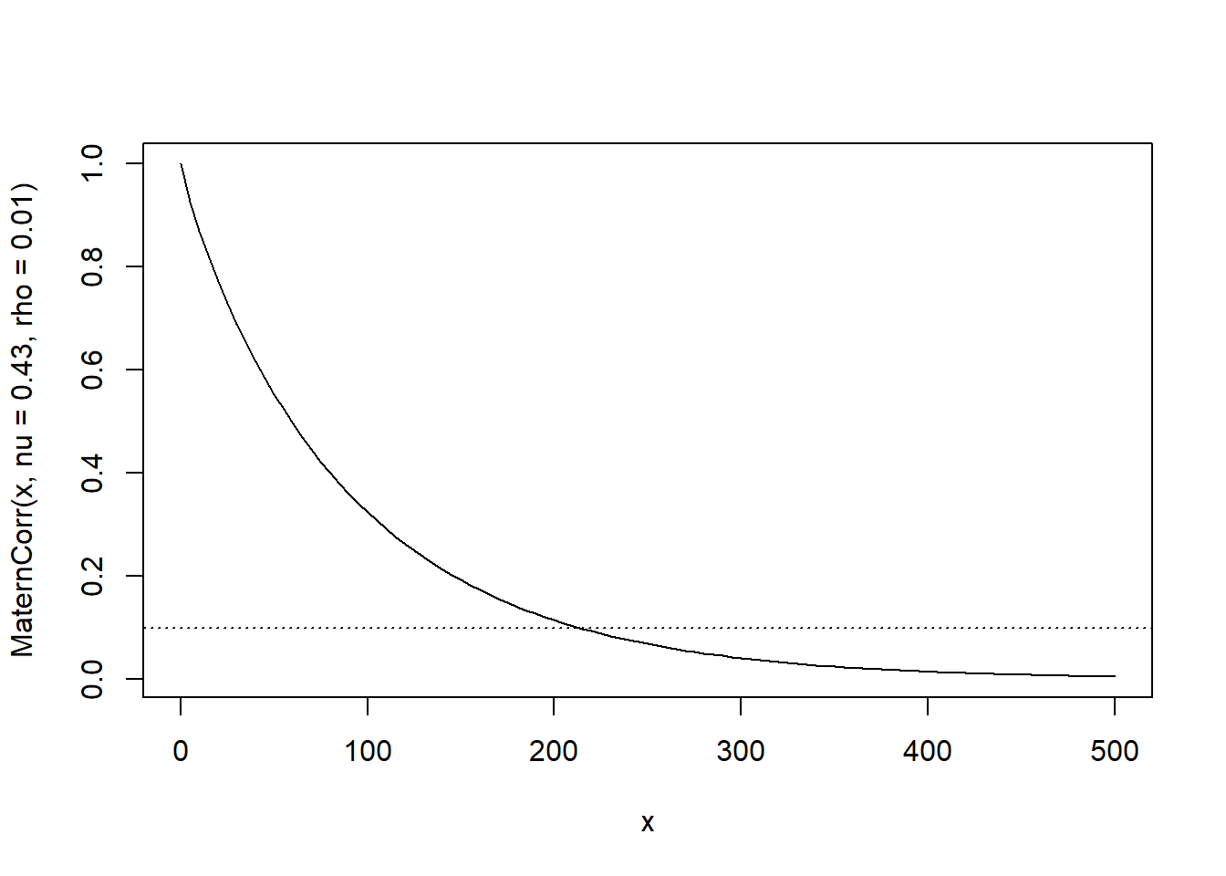
The \(\nu\) is quite close to 1/2, so the spatial correlation is approximately exponential. Note that even at 200 m distance, there is still something like a 10% correlation in the residuals.
3.4 Crazy prediction plot
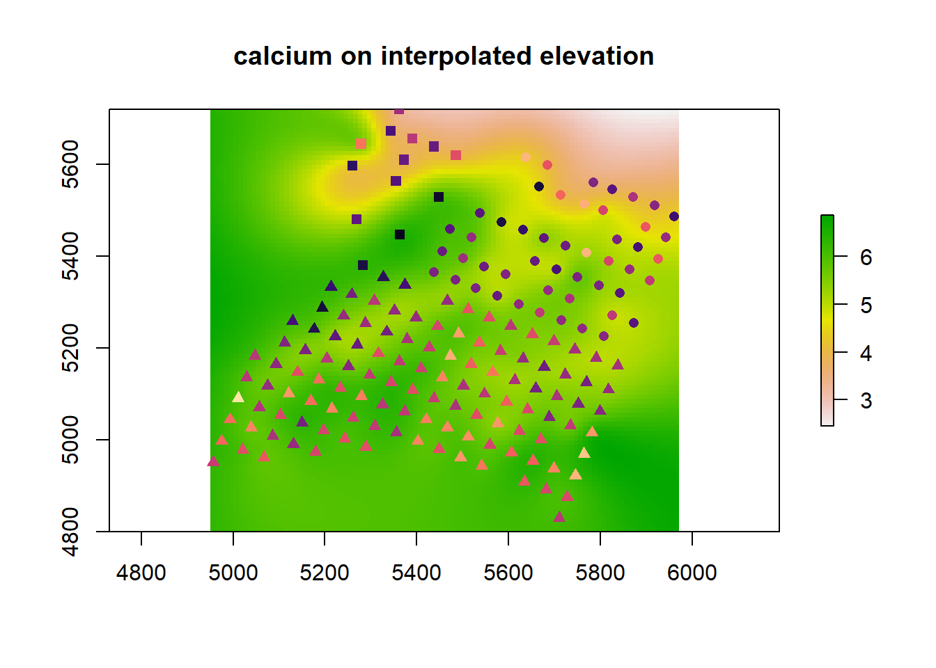
This is a terrific plot. The code was cheerfully stolen from this blog post.
library(fields)
library(raster)
# derive a DEM
elev_m <- Tps(dat[,c("x","y")], dat$elevation)
## Warning:
## Grid searches over lambda (nugget and sill variances) with minima at the endpoints:
## (GCV) Generalized Cross-Validation
## minimum at right endpoint lambda = 5.669116e-06 (eff. df= 169.1 )## Warning:
## Grid searches over lambda (nugget and sill variances) with minima at the endpoints:
## (GCV) Generalized Cross-Validation
## minimum at right endpoint lambda = 5.669116e-06 (eff. df= 169.1 )
r <- raster(xmn = 4950, xmx = 5970, ymn = 4800, ymx = 5720, resolution = 5)
elev <- interpolate(r, elev_m)
# for the region info use the limits given in ca20
pp <- SpatialPolygons(
list(Polygons(list(Polygon(ca20$reg1)), ID = "reg1"),
Polygons(list(Polygon(ca20$reg2)), ID = "reg2"),
Polygons(list(Polygon(ca20$reg3)), ID = "reg3")))
region <- rasterize(pp, r)
# predict at any location
newdat <- expand.grid(x = seq(4960, 5960, length.out = 100),
y = seq(4830, 5710, length.out = 100))
newdat$elevation <- extract(elev, newdat[,1:2])
newdat$region <- factor(extract(region, newdat[,1:2]))
# remove NAs
newdat <- na.omit(newdat)
# predict
newdat$calcium <- as.numeric(predict(m_spamm, newdat))
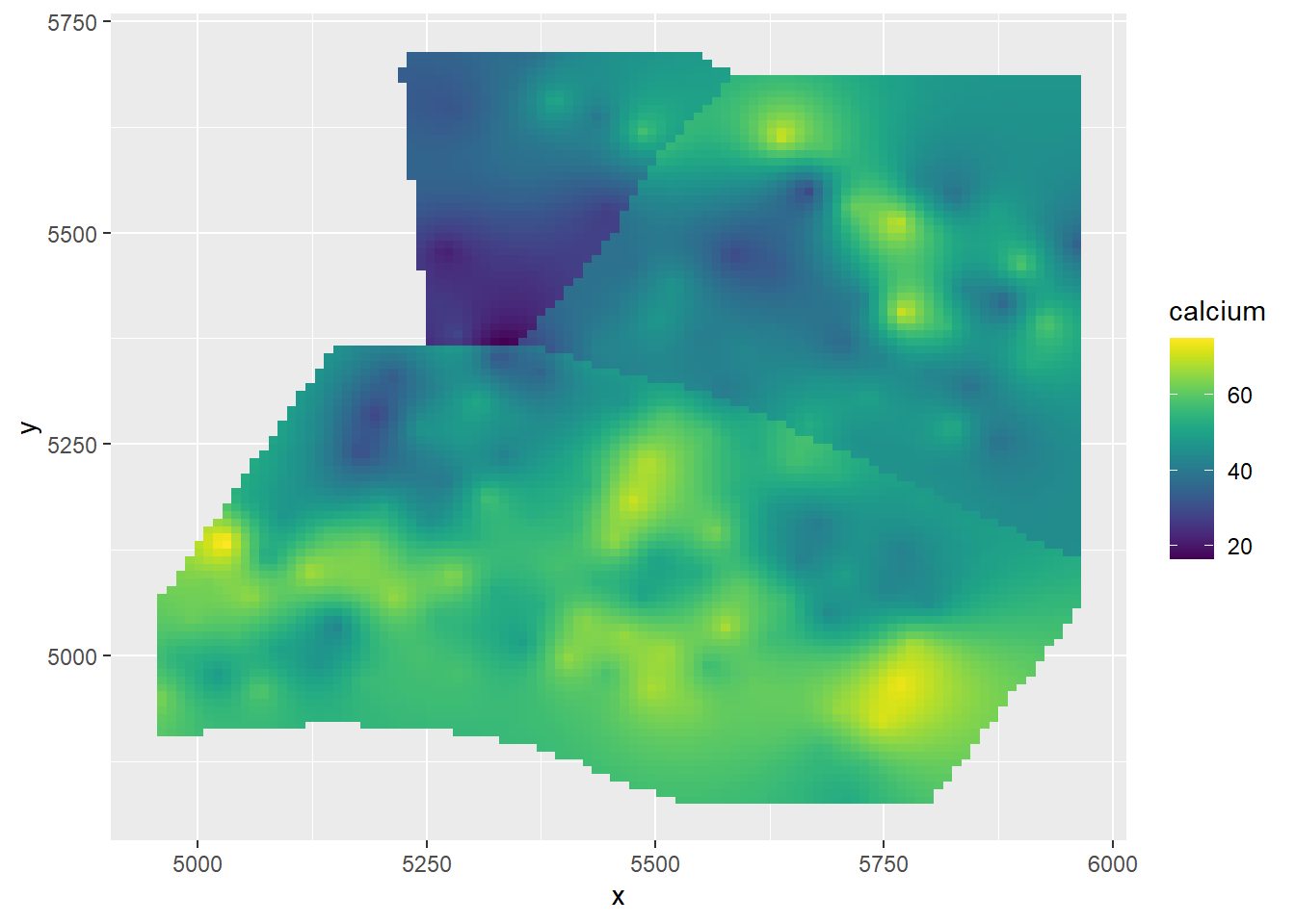
(gg_spamm <- ggplot(newdat,aes(x=x, y=y, fill = calcium)) +
geom_raster() +
scale_fill_viridis())