This is my first blog post on this site. It is therefore, in large part part, an experiment to see if this whole blogging mechanism works. Foolishly, it is a long post, and an ambitious one (technically speaking). Also - foolishly - it is laden with both content and context.
The context is that I’ve spent too much of the past few days trying to answer a question that I thought would be fairly straightforward. Now that I have a solution - which is only mostly satisfactory, it seems it will make the overlong journey more worthwhile to record some of the twists and lessons along the way (never mind that it took an additional few days trying to get this blog to post!). There are some fun themes here, of randomness, contructing null hypotheses, spatial point processes, and a teeny bit of R code. In the end, I have a tool which (I hope) will be useful to getting real insights into animal behavior (in this case - caribou), but that might be of broader interest as well. Perhaps others can suggest better ways to get there (assuming the comments feature below works!)
The context
I spend a lot of time studying movement data on caribou in North America. Caribou are mysterious in many, many ways, and there are many unique challenges in analyzing their data - grist for many (almost surely never-to-be-written) blog posts. Not least of these challenges is that in a herd that can contain many tens of 100’s of thousands of animals - there are usually around 20 animals collared at a time. At best - 50-ish. So broad inferences have to be made (carefully) from very small samples.
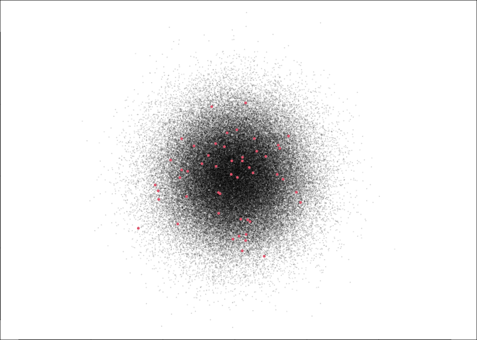
This, for the record, is what 50 (red) points out of 100,000 looks like:
And this is what congregating caribou look like:

(Image by K. Joly - from a recent paper published, unexpectedly, in the journal Toxins).
Obviously caribou are social and aggregate. The question is: if we only observe only very few of them, can we detect significant social aggregation? And - more relevantly - see how those aggregations vary over time?
A super-straightforward estimate
Let’s take a look at a very straightford measure: how many really close encounters are there in some subset of data? Below, a figure of the number of pair-wise distances among all caribou (from one particular herd, in one particular year) that are less than 200, 100 and 50 m. Note - the range size for this particular herd is on the order of 100’s of km in a given dimension, so these distances are really quite small.
Ok, here’s the graph:
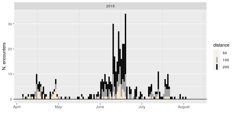
A lot of variation here - plenty of days with no animals within those encounter radii, and then some days when there are 30 or more close encounters. And a lot of biologically interesting patterns. For example, inter-individual distances are (surprisingly) very low during the spring migration period (essentially - May), peak during the early summer calf-raising period, but are much lower during late summer.
Let’s zoom in on just a 10 day period and see what’s going on. The red croses indicate pairs of animals within 200 m of each other, with the count (in red) at the bottom of each panel. The grey blob indicates the 80% kernel density of the complete set of points (which neatly excludes those animals that are far off to the north):
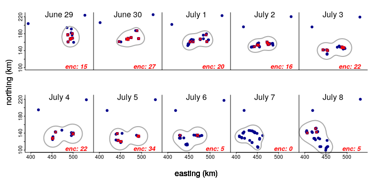
Two things to note: The size of the blob stays pretty constant - and the number of individuals is the same. But the number of encounters varies A LOT, peaking at 27 on June 30 and crashing to 0 a week later on July 7.
Again - there’s a super interesting behavioral question here, and intriguing ecological hypotheses to explore. But the main question here is statistical, namely: are those numbers of encounters more than expected? Are others less than expected? Can we get to that oh so hotly desired crutch of all inference … a p-value from these observations?
Some point processes
Before we get to a p-value, it’s helpful to simulate data so we can really, really know what’s going on. I used various random point-generation functions in the package spatstat to create three distributions of 32 points each, just as with the caribou data above:
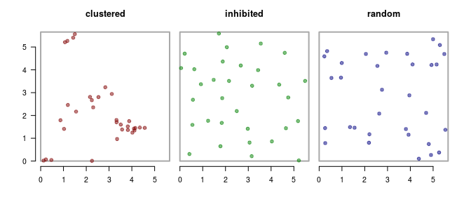
The “clustered” process looks like there are a bunch of aggregations. The “inhibited” process looks like everyone is a superchamp social distancer. The third one - is, well, perfectly random (which - maybe to many people - looks like it’s bunched up in funny ways, but that’s to be attributed to our miserable human intuition for randomness).
If we count the number of encounters - which we’ll defined as the number of unique pairs less than 0.3 units distance of each other, we get the following results:
- clustered: 28
- inhibited: 0
- random: 4
So the “random” number is a Goldilocks number, not too few, not too many. And the process that generated it a decent working null hypothesis. That process is complete spatial randomness (sometimes CSR), or, more wonkily, a homogeneous spatial Poisson point process. This is quick to generate, and quick to summarize, so a super straightforward approach is just to simulate the process a bunch of times and count the encounters.
I don’t - generally - want to clutter these blog posts (note how ambitiously I anticipate future posts!) with too much R code, but the following code is maybe worth sharing (despite the horrors of a loop!) because it relies entirely on very “base” functions:
getNwithinR <- function(z, r){
  D <- outer(z, z, function(z1,z2) Mod(z2-z1))
  sum(D[upper.tri(D)] < r)
}
density <- 1;  n.ind <- 32;  area <- n.ind/density
N.enc.null <- rep(NA, 1e4)
for(i in 1:length(N.enc.null)){
      z <- runif(n.ind, 0, sqrt(area)) + 1i*runif(n.ind, 0, sqrt(area))
      N.enc.null[i] <- getNwithinR(z, .3)
}
Here’s the resulting histogram, with our three observations (inhibited, random, clustered):
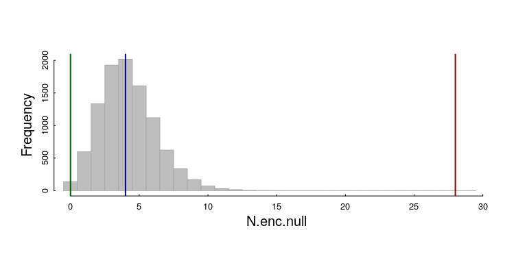
We can get pretty precise empirical (randomization) p-values on our three observations: The 28 encounters in the clustered pattern (red line) is WAY HIGHER than expected: $p$-value = 0. The p-value on the inhibited pattern (with 0 observations) is also not too likely, though the probability is at least detectable: 116 of 10000 simulations for a p-value of 0.0116. The random result is slap dab in the middle of the null distribution.
Analytical results!
Randomization can get you really, really far in inferential life. It is, unfortunately, not really practical with very large amounts of data. And, it turns our, we can - with not too much difficulty - derive a formula that takes the number of individuals (n), an area of use (a), and an encounter radius (r) to provide a good null distribution, against which observations of encounters can be compared.
The homogeneous Poisson process is defined by only one parameter, $\lambda$, called the intensity (generically). In two dimensions, the intensity is just the density of points. That’s the process, but the statistic we observed is the Number of Encounters, given r, a, and n (let’s call that $E_{total}(r,n,a)$), and the real question is how is THAT random variable distributed.
The trick is to think of the pair-wise encounters as (independent) events, and compute their probability. The number of unique pairs is n(n-1)/2 … that’s maybe most easily seen as the upper triangle of a matrix of all links:
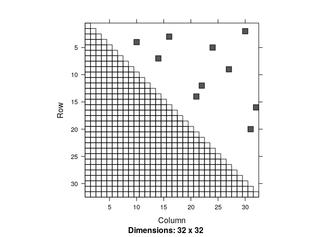
Every cell of the (upper half) of this matrix represents one pair-wise link among 32 individuals, and - in this case - the smattering of dots represents those pairs whose distance is less than 1. Those pairwise distances are (and this is a very important point) are themselves completely random. And their probability is easy to calculate. If you randomly pick a point in space - anywhere - the probability that another individual is within radius r of that point is the area of a circle or radius r divided by the total area a, so: $p = \pi r^2 / a$.
So the distribution of the number of unique encounters is just the sum of a bunch of (low) probability events of probability $p$ over $n(n-1)/2$ possible pairs, i.e. a Binomial distribution, with the two parameters $p = \pi r^2 / a$ and $n’ = n(n-1)/2$. This is a really easy distribution to work with!
\[E_{total}(r,n,a) \sim Binomial\left(\pi r^2 / a,\ {n(n-1)\over2}\right)\]Furthermore, if $p$ is very small (which is generally will be) and $n’$ is reasonably large, which it outght to be, we can approximate it as a Poisson distribution, with intensity $\lambda = p n’$, so, to a very good approximation:
\(E_{total}(r,n,a) \sim Poisson\left(\lambda = {\pi r^2 \, n(n-1) \over 2 a}\right)\) The expected value (mean) of both of these distributions is $\lambda$.
A very tidy and simple result! Let’s compare these with our simulated result:
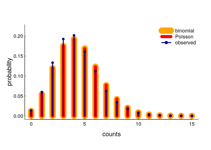
You can see pretty darned good correspondence (the binomial and Poisson models are indistinguishable), though there is a slight shift towards fewer observations than predicted. In fact, the expected number of encounters (according to our model - with n = 32, r = 0.3, area = 32) is 4.38, whereas the actual (simulated) mean is somewhat lower at 4.21. This is almost certainly because of edge effects: points closer to the edge of the area are somewhat less likely to have a close neighbor. But, that seems like a minor effect (and certainly a very difficult one to correct for).
Revisiting the data
So … we now have all the tools needed to apply a statistical test to observations of encounters! The steps are as follows:
- Find all of the encounters on a given day for a given radius.
- Compute a “ranging area” (which - in the most hand-wavy bit of this analysis - I’ll set to an 80% kernel density estimate … because I know using my familiarity with the data and all-powerful and too-little-used “biological intuition” that there are always a few stragglers and idiosyncratic, free-thinking ne’er-do-wells in every animal population that are best left out of the whole computation).
- Use the binomial distribution under the null assumption of random uniform distribution within that ranging area to obtain an expected number of encounters and a p-value for (either) the hypothesis of too few encounters, or too many encounters.
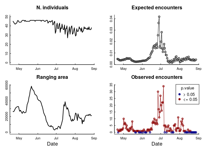
Here’s how that looks:
What to make of this!?
There are a few things to unpack here. The “ranging area” - as inferred from this group of individuals - fluctuates a LOT over these months, and the peak of encounters corresponds to a period in late June / early July when that area is particularly small (about 3000 km$^2$ compared to over 30,000 km$^2$).
Most dramatically: the expected number of encounters is VERY VERY SMALL! It never even reaches 0.1. That means that even a single close encounter is going to be statistically significant, and 30 encounters is astronomical. The variation in that curve, however, is very interesting, as it does reflect that shift in total range area, but they don’t entirely line up - and that plummeting cliff in the number of encounters is unexplained by that variation.
This suggests that the “forces” that drive the caribou - in general - to a smaller area might also be related to forces that drive caribou to become exceptionally “close,” though the immediate drivers of high encounters remain unexplained (though we have some ideas!).
More relevant to this post, these results do strongly suggest that even a rather small sample of data from an enormous population is enough to reveal a very, very strong signal of social aggregation, which (frankly) I didn’t necessarily expect. On the other hand, it is important to consider whether the null hypothesis is just too unrealistic. It might be that the 80% kernel density is just too darned large, though even picking a very small core range won’t affect the results that much. It also might be that spatial randomness is not the best way to distribute null points, that it would be better to account for higher densities in core areas of the range. That could have a stronger effect, though it would be hard to know how to generate a null distribution from an inhomogeneous process, or to trust any inference from the idiosyncratic sampling on higher-level properties of the distrubution.
It is likely, for example, that not all space within the “ranging area” is similarly available and that there are topographic and geographic features which will tend to cluster the caribou. I am a little bit familiar with the portions of the Canadiand Arctic that these animals hail from … and, while there are NO mountains or valleys, there might be significant patches which are simply too barren to be of any use. To account for that, we would need a good resource selection model as a foundation for the null distribution. This is a whole step more complex but - in this context - perhaps a worthwhile direction to pursue.
But, for now, I think the Binomial Aggregation Distance test (BAD) is - well - not too bad for these purposes.
(Sorry about that. I should quit while I’m ahead.)