An interesting question came up the other day from a colleague who is modeling the spatial interaction between two animals (caribou and muskox) whose ranges overlap in a study area in a portion of the Canadian Arctic. She has fitted two resource selection functions (RSF’s) - one for the caribou, one for the muskox - identified some relevant differences in their preferences for different elevations, vegetation types, distance from water, etc., and is now wondering if she can use those results to create a map of “co-occurrence” of the two species on the landscape. This question is not entirely abstract - there is local concern in this particular region that the muskox (which had been extirpated and more recently reintroduced) are competing with the caribou, which are an important local resource for subsistence. The socio-ecological context - as always - is interesting and complicated. But the statsy question itself is also interesting, as it forces us to think about what does an RSF really tell us, and what does co-occurrence really mean.
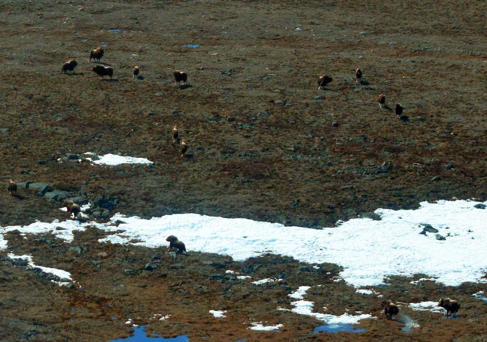
Muskox are amazing. When you see them, they look like paleolithic aliens that have been teleported from Pluto. Here are some that I saw on a caribou survey (photo: Dean Cluff).
An aside to grumble about RSFs
To be honest, I have some (maybe many) issues with RSF’s, even though I have dealt with them quite a bit (here’s even a link to a series on primers), especially when applied to movement data. They can be useful for generating easy to interpret maps of habitat suitability, and for identifying some general patterns of preference or avoidance, and those maps have real value, both for communication and decision-making. And, since movement data from GPS collared animals is one of the most commonly available kinds of data for “observing” animals in the wild, it is tempting to use those data to make habitat suitability maps - as well as some inferences on habitat-specific preference or avoidance.
However, there are a lot of weird assumptions that underly them. For example: that an animal walking around a landscape has a bird’s eye GIS-layer type knowledge of accessible habitats and can spread itself around space. Or that an “availability” set - which is usually just sampled randomly from some landscape - meaningfully reflects “lack of use”. Also, in my experience, RSF’s are just fussy and slippery and (computer) resource intensive.
Finally, a problem with RSF’s is confusion regarding how to interpret the predictions. You perform some kind of logistic regression, which gives predictions on a “logit” (or log-odds) scale, which - in a normal logistic regression - you can just convert to a probability. But probabilites aren’t really meaningful if you yourself artificially set the availability data set! If you have as many available points as used points, the overall probaiblity is 1/2. If you have 10 times as many “available” points, it is 1/11. So rather than back-transform, RSF’s are usually defined as JUST the exponential bit.
All that said, my own interpreration of RSF’s has been very enjoyably “paradigm shifted”1 by some recent reinterpretation of RSF’s in terms of point process intensities. And that reinterpretation really helps answer a question like this one. Though - as usual - there were a few unexpected twists along the way.
Point processes
But first … what does “co-occurrence” for a bunch of points in space?
In theory - a point takes up zero space. So the probability that two points “co-occur” is, most strictly speaking, zero. So the question only means anything in terms of some area of co-occurrence (or alternatively, but really very similarly, some distance of interaction). At the scale of the study area in question (the portion of the Canadian Arctic with caribou and muskox) co-occurrence is 100%, and at the extreme spatial scale of the entire world, we are all co-occurring. While that makes for a terrific bumper sticker-worthy sentiment, it’s not actually that useful.
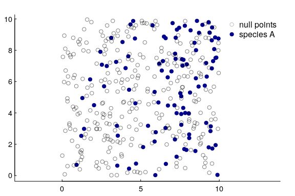
So let’s go back and think about points. Below, we have two species, 100 individuals each, sharing 100 squared units of space. The density of each is 1 animal per unit squared, but the spatial distribution is completely random.
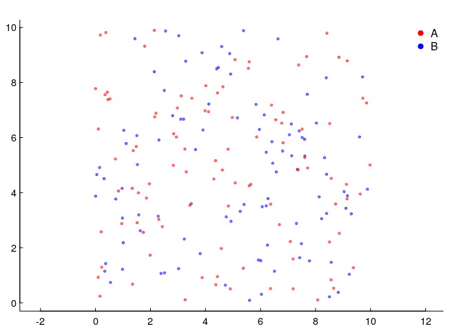
This is the simplest (homogeneous) two-dimensional Poisson point process. Why Poisson - which many associate with a discrete distribution frequently used to model count data? Because if we subset the space equally, the number of these points per unit area will be distributed as a Poisson random variable. Here’s an illustration, where we took the data above and broke it down into 100 square units and counted the number of red and blue points in each.
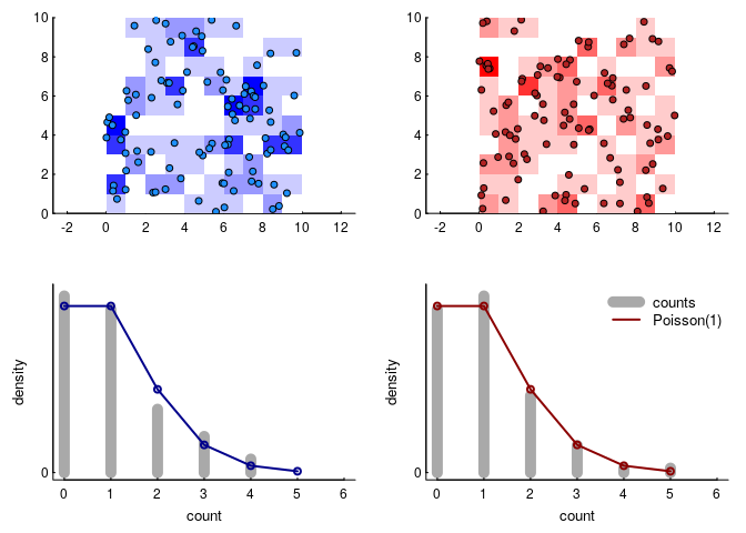
Because the intensity parameter is equivalent to the mean density of points, $\lambda = 1$ and the resulting count distribution is a Poisson distribution with intensity 1. We can write that in terms of the density function as: \(P(A = k, \lambda_a) = {\lambda_a^k e^{-k} \over k!}\).
Co-occurring point processes
We can define co-occurrence - reasonably - as the probability that there is at least one of both species in a given cell. This definitian is, of course, contingent on the area of that cell. We might write that something like: \({\cal C_{occ}} = P(A \geq 1|\lambda_a) \, P(B \geq 1|\lambda_b).\) The probability that there is at least one of something is, conveniently, equal to 1 minus the probability that there is none of that something, so the probability of co-occurrence is \({\cal C_{occ}} = (1 - P(A = 0)) \, (1 - P(B = 0)) = (1 - e^{\lambda_a})(1 - e^{\lambda_b}).\) Note, we’re letting the $\lambda$ be unique for each of the two species.
This is a nice tidy result. In our case, $(1 - 1/e)^2 \approx 0.4$ and, sure enough, there are 38 out of 100 co-occupied squares in the simulation.
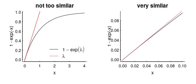
Even more conveniently, if $\lambda$ is very small (which would happen if, say, the area of our squares were smaller, or the density of points were lower), then $1 - e^\lambda$ looks an awful lot like just $\lambda$, which is an even more convenient result, because it just says that the co-occurence probability is $\lambda^2$.
The intensity / density parameter $\lambda$ captures the general likelihood of an animal being found in a general location. It is “scale robust”, because it is a nice, useful, meaningful measure despite the fact that the probability of being in any one (infinitesimally small) location is always 0, and being anywhere in the universe is 1.
So, in a very similar way, that $\lambda^2$ (which has weird units of density² - or, e.g., $n_A n_B/km^4$) is a legitimate measure of “co-occurrence intensity” that can be considered similarly “scale-robust” and meaningful for any location in space.
What does this have to do with RSF’s?
The “paradigm shift” I alluded to earlier is to abandon any pretense or interest in RSF’s as modeling a probability (as McDonald 2013 would suggest - don’t even think of RSF’s a a “logistic regression” at all), or even as a “weighted spatial distribution” (as per. Lele and Keim 2006), but to embrace them as an estimate - specifically - of the spatial intensity of an inhomogeneous Poisson process, i.e. as spatially explicit estimates of $\lambda$ above.
I’ll unpack this a bit below, but really, I can’t recommend enough this excellent video lecture by John Fieberg at this link, also associated online materials here, especially Fieberg’s slides. It’s an “introductory lecture”, but one that presents the RSF machinery explicitly in the context of inhomogeneous point processes (what Fieberg rightly calls “The Great Unifier”).
So, when we fit RSF’s we ususally have a Used / Available (ideal would be “Not Used” … but that’s far too rare) design where environmental variables are collected for the observed set and the “available” set, which is usually some sort of sampling reflecting some sort of null hypothesis. We then do what looks like a logistic regression, which fits the following model
\[P(Y = 1) = {\exp(\beta_0 + \beta_1 X_1 + \beta_2 X_2 + ...) \over {1 + \exp(\beta_0 + \beta_1 X_1 + \beta_2 X_2 + ...)}}\]where the $X_i$’s are the covariates we think are useful predictors, and the corresponding $\beta$’s are the regression coefficients. Positive values of $\beta$ indicate higher probabilities of use, negative values indicate lower probabilities of use.
However, since we are not actually interested in probabilities (e.g. in the intercept of the logistic regression above), the Resource Selection Function itself is usually just defined on the numerator, with the intercept simply tossed out:
\[w_i(x, \beta) = \exp(\beta_1 X_1 + \beta_2 X_2 + \beta_3 X_3 + ...)\]This has the advantage of being simpler to look at, but opens up the question of what is $w(x,\beta)$.
So, bypassing other interpretations, approaches and debates, the bit of weird, deep, almost magical insight is that if you give the “available” subset arbitrarily large weights, the function $w$ leads directly to a a good estimate of $\lambda(x)$! Specifically: \(\widehat{\lambda}(x) = {n \, w(x, \beta) \over \int_A w(x, \beta) \, dx}\)
Let’s illustrate this. We’re going to simulate species $A$, but with a single covariate that’s just the $X$ coordinate, i.e. the points are more concentrated to the east than in the west:
Now, I know the density increases linearly with x, and to capture that we actually have to fit the logistic regression against $\log(x)$ as the covariate. This is a strong argument, by the way, for taking the log transform of any “distance-to” variable in an RSF if you want to model a linear relationship between densities and distances, AND if you want the density to be 0 at the 0 edge. Otherwise, that modeled relationship will always increase exponentially, which causes all sorts of problems.
Below, in a few lines of code, I simulate the inhomogeneous point process and fit the model. NOTE the arbitratily high weight (1000) for the null locations, even though in reality I have the same number of both null and available:
z1 <- 10 - 10*rbeta(100, 1, 2) + 1i*runif(100, 0, 10)
null <- runif(300, 0, 10) + 1i*runif(300, 0, 10)
df <- rbind(data.frame(Used = TRUE, X = Re(z1), w = 1),
      data.frame(Used = FALSE, X = Re(null), w = 1000))
fit1 <- glm(Used~log(X), weights = w, data = df, family = "binomial")
summary(fit1)$coef
##              Estimate Std. Error    z value     Pr(>|z|)
## (Intercept) -9.826814  0.3838600 -25.599998 1.52561e-144
## log(X)       1.140449  0.2049926   5.563366  2.64620e-08
The estimated coefficient on the $\log(X)$ variable is 1.14 (se. 0.2). By making the equivalence between that (intercept free) exponential bit and the intensity function, the inhomogeneous intensity $\lambda$ (recall, inhomogeneous here just means a function of x and y): \(\widehat{\lambda}(x,y) ={ n \, \exp(\beta \log(x)) \over \int_0^{Y} \int_0 ^ {X} \exp(\beta \log(x)) \, dx \, dy}\) where X and Y are the dimensions of the rectangular area. For this particular log-distance model, the whole thing breaks down into the following result:
\[\widehat{\lambda}(x,y) = { n \, x^\beta \over Y \int_0^X x^\beta \, dx} = {1 + \beta \over A} \left({x \over X}\right)^\beta n\]where $A$ is the overall area XY.2
You can see our prediction below against the observations:
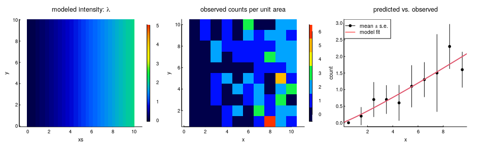
It’s a good model! And it shows how to directly link an RSF result to an intensity / density.
Nice RSF, but what about co-occurrence?
We’re just about there.
Here’s another - final - simulated data set. In this version, there are two species: 100 muskAxe (A) and 400 cariBoo (B)3. They have somewhat different responses to two covariates, which (for simplicity) are again just the geographical coordinates X and Y. Specifically, the muskaxes are more likely to be found towards the north and east, and the cariboos are concentrated near the south - in both cases in somewhat non-linear ways (quiet shout-out to the all-versatile Beta distribution). We’ll put these animals on a raster, which has 100 m x 100 m resolution over an area of 100x100 km².
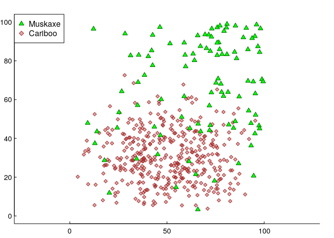
We fit some (logistic) GAM’s, with, say, 1000 uniformly sampled null points from the availability set
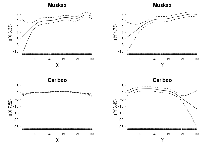
In an RSF analysis, usually people work with rasters of the covariates (in this case, just X and Y values). We can convert our GAM’s in a surface of intensities with the following steps:
- (a) predict over the raster,
- (b) subtract away the intercept and place that in the exponent (that’s $w$),
- (c) “normalize” that $w$ by dividing by its sum and multiply by the grid-cell size $\Delta x \Delta y$4
- (d) multiply the whole thing by the number of total individuals.
The code will look something like this:
A.intercept <- glm.A$coefficients[1]
B.intercept <- glm.B$coefficients[1]

w.A <- exp(predict(xy.brick, glm.A) - A.intercept)
w.B <- exp(predict(xy.brick, glm.B) - B.intercept)

lambda.brick[[1]] <- w.A/(sum(getValues(w.A)) * res(w.A)[1] * res(w.A)[2]) * n.A
lambda.brick[[2]] <- w.B/(sum(getValues(w.B)) * res(w.B)[1] * res(w.B)[2]) * n.B
And the resulting density predictions:
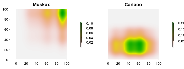
We can confirm that the numbers are “correct” by making sure that the mean densities are 100 ind./(100 km x 100 km) = 0.01 and 400 ind./(100 km x 100 km) = 0.04:
mean(getValues(lambda.brick[[1]]))
> [1] 0.01

mean(getValues(lambda.brick[[2]]))
> [1] 0.04
Looks good!
Finally, we’re ready to plot a co-occurrence intensity plot, and all we have to do is multiply the two intensities!
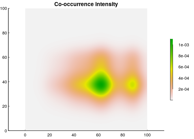
This, then, is a map of the “intensity” of co-occurrence, which - again - is in weird units of ind² / km⁴, but is actually a fairly straightforward measure. It says that per km², you can expect at most about 0.0016 muskax and cariboo to share that unit of space (compared to an over-all co-occurrence density of 0.004). Or - you can state that as a probability (and expand the geographic range) and say that in a 10x10 km² area, the probability of encountering at least one cariboo and muskax peaks at something like 16%.
Note that this co-occurrence intensity is weighted more towards the cariboo; a reflection of the fact that there are 4 times more caribou in the data. However (and this is very important) presumably, what’s of actual interest is co-occurrence across the entire population. And for that, you need an important piece of information that is not always availble, namely the population estimate of each species!
With that important piece, one can now take two (or more) RSF’s and turn those into a co-occurrence intensity map. Easy peasy.
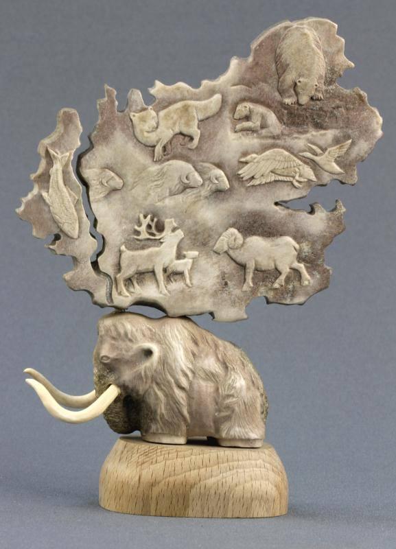
Higher order multi-species Arctic megafauna co-occurrence, at least in the imagination of a carved woolly mammoth, is illustrated below.5
-
Can paradigm shifts even be personal? ↩
-
Actually - we know that the “true” answer is $\beta = 1$ (which fits within the standard error of the regression estimate), which makes the whole thing reduce to simply: $\widehat{\lambda}(x,y) = {2n \over AX} x$, i.e. a linear density that ranges from 0 to $2n/A$, averaging out to $n/A$. ↩
-
Out of something resembling principle, I refuse to give simulated animals names of actual species! ↩
-
recall that the discrete version of $\int_0^{Y} \int_0 ^ {X} f(x,y) \, dx \, dy = \sum_{i = 1}^{n_x} \sum_{i = 1}^{n_y} f(x,y) \Delta x \Delta y$ ↩
-
With an essential shout-out to the anonyous carvers from Taymir, Russia … this picture came from somewhere within this website: http://www.tdnt.org ↩