Circumpolar mapping (by Chloe Beaupré)

It’s been over three years since a blog post. Does that even count as a blog? Since the last entry, I’ve become a professor. Which (a) takes a big old chunk out of time to do anything else, but (b) provides access to a hitherto unavailable resource known as graduate students (a subset of the spectacular lab members phenomenon). One of these, Chloe Beaupré, provides the following hot tips for dealing with some very particular mapping issues in R.

background

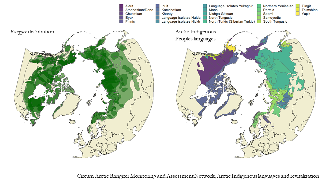
For a presentation I wanted to create a plot of the Arctic, showing the circumpolar distribution of Rangifer populations next to a map of a map of Arctic Indigenous languages. Turns out mapping a circumpolar projection in R is not as easy a making a pretty map of a smaller area at lower latitudes. Here is an outline to recreate (one of) these plots.

packages <- list("dplyr","sf", "ggplot2","mapview", "viridis","maptools", "raster")
sapply(packages, require, character = TRUE)

shapefiles

We’ll plot the map of arctic Indigenous Peoples languages and dialects since the data are made publicly available by the Arctic Indigenous languages and revitalization project. Shapefiles can be downloaded here.

After downloading the shapefiles, read them into your environment and re-project to the EPSG 3995 projection (arctic polar stereographic) using the sf package

lang <- st_read("data/Arctic_Indigenous_Peoples_languages_and_revitalization_-_Languages_and_Dialects.shp") %>%
  st_transform(st_crs(3995))

mapview fails us

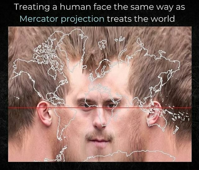
We usually love plotting spatial data using the mapview package because it’s fast and interactive but it defaults to the dreaded Mercator projection.

mapview(lang)

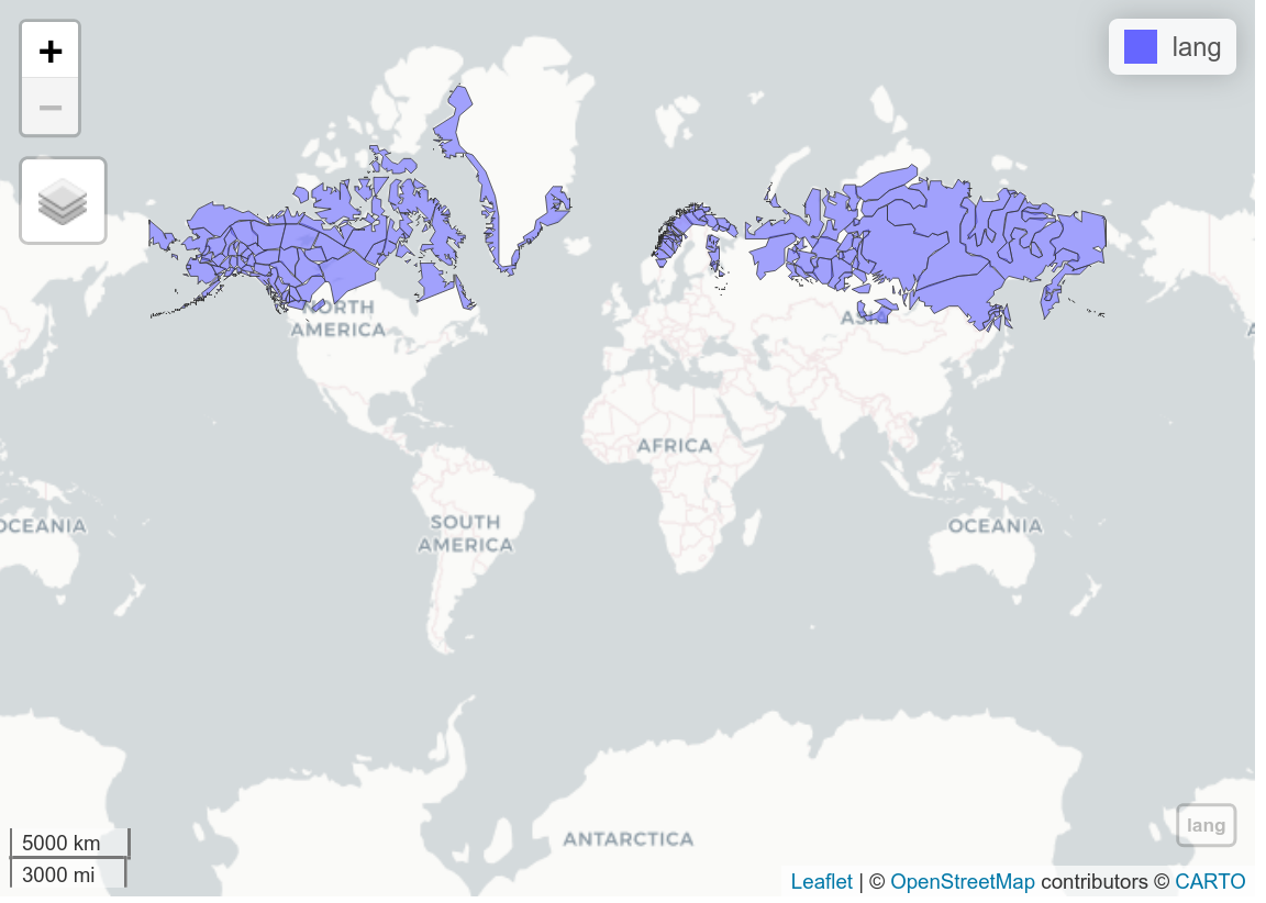
[ed. note - interactivity of mapview disabled on blog]

Looks horrifying.

There is an argument in mapview to use the native CRS (which we’ve transformed to Arctic Polar Stereographic EPSG 3995), let’s try it out.

mapview(lang, native.crs = TRUE, map.types="Esri.WorldImagery")

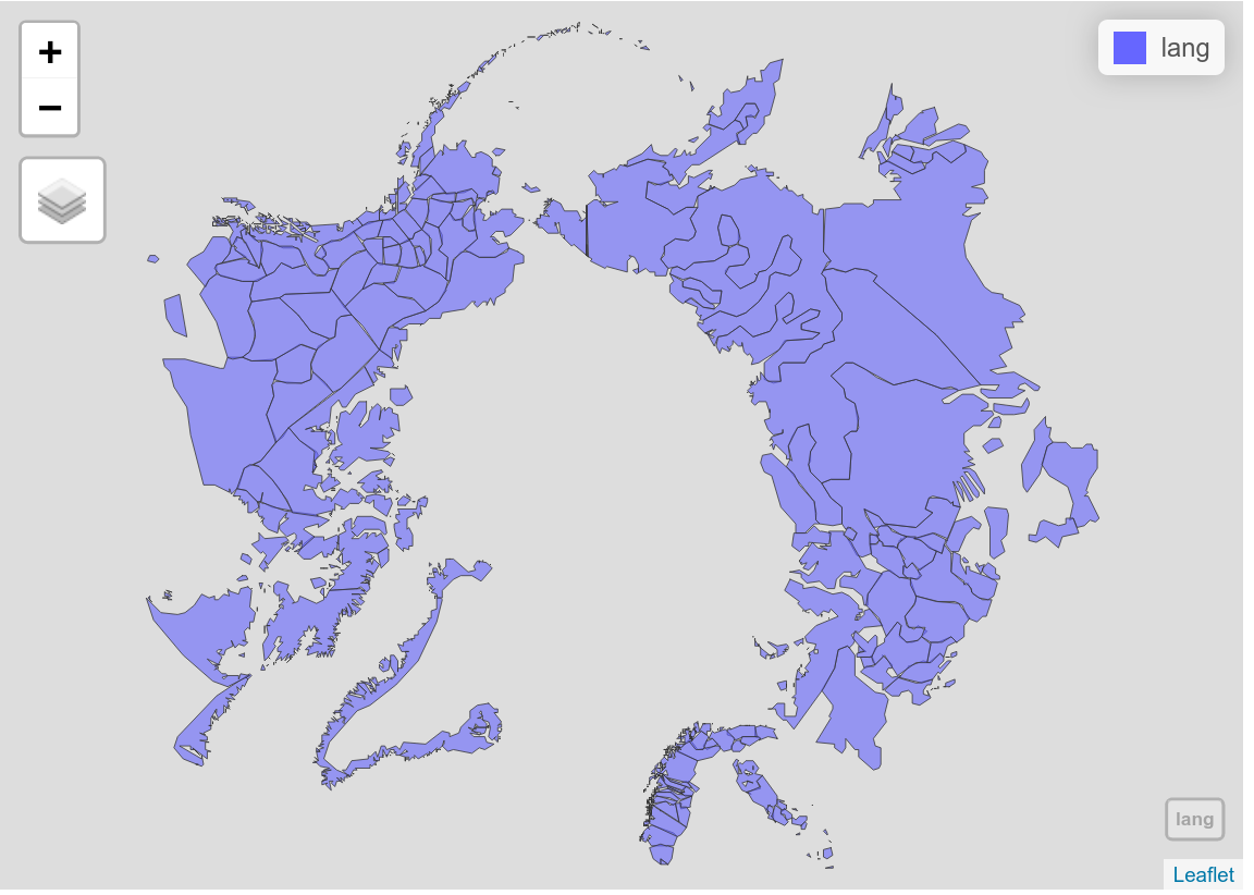
This looks better! But there isn’t a basemap for the North Pole so we have our language polygons floating in the ether. We can do better.

coastlines

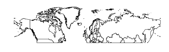
The maptools package provides a simple whole-world coastline data set. We set the y-limit to 45 degrees North, so only keep the coastlines in the north.

data("wrld_simpl", package = "maptools")                                                                            
w <- raster::crop(wrld_simpl, extent(-180, 180, 45, 90))                                                                   
plot(w)    

After downloading the northern coastlines, convert to a simple feature multipolygon, then re-project to the arctic polar stereographic (EPSG 3995).

# make it into an sf object, transform the crs
w_sf <- w %>%
  st_as_sf(coords = c("long", "lat"), crs = 4326) %>%
  st_transform(st_crs(3995))

putting it all together

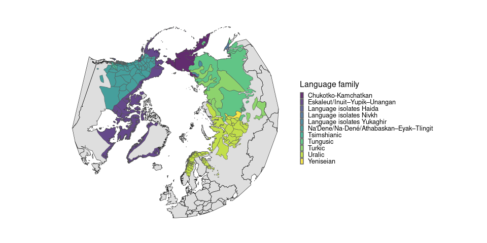
The following code uses ggplot2 to plot the arctic coastlines and overlays the arctic Indigenous Peoples languages shapefile.

ggplot() + 
  geom_sf(data=w_sf, fill = "grey", colour = "black", alpha = 0.5) +
  geom_sf(data = lang[!is.na(lang$LangFamily),], aes(fill = LangFamily), alpha = 0.8) +
  scale_fill_viridis_d()+
  scale_x_continuous(breaks = NULL) +
  labs(title = "", x = "", y = "", fill = "Language family") +
  theme(axis.text = element_blank(),
        axis.ticks = element_blank(),
        panel.background = element_blank(), 
        text = element_text(size = 12),
        legend.key.size = unit(.2, 'cm')) # make the legend smaller

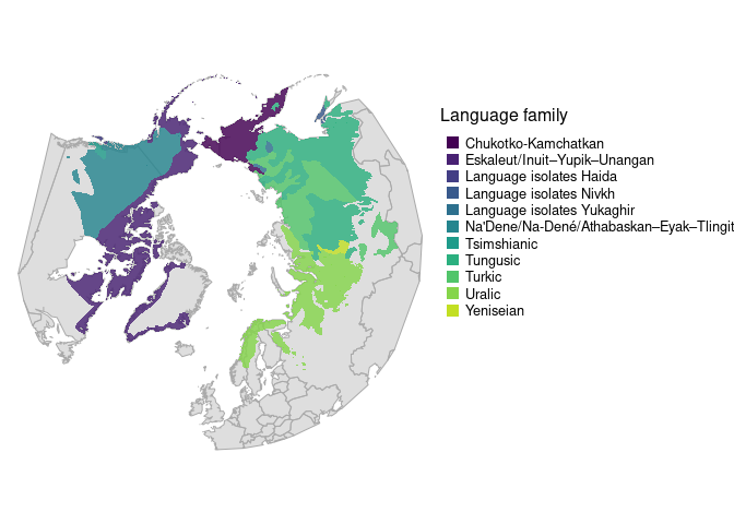
The remaining code creates a similar plot using base R if that’s more your style (cough owner-of-this-blog-Elie cough).

cols <- viridis(n = length(unique(lang$LangFamily)))
labs <- levels(as.factor(lang$LangFamily))

# set margins
par(mar = rep(.1,4))
layout(matrix(1:2, ncol =2), widths = c(1.5,1)) 

# plot the coastlines, to initiate the area
plot(st_geometry(w_sf), lwd=1, lty=1, col= alpha("grey", .5), border = "darkgrey")

# plot the language data
plot(lang["LangFamily"], lwd = 1, lty = 1, pal = alpha(cols, .8), add = TRUE, border = NA)

par(mar = c(0,0,6,0), xpd = NA); plot.new()
mtext(side = 3, "Language family", font = 1, line = 0, adj = 0)
legend(x = "topleft", ncol = 1, cex = 0.8, legend = labs, col = cols, pch=15, pt.cex = 1.5, bty = "n")

• Chloe Beaupré

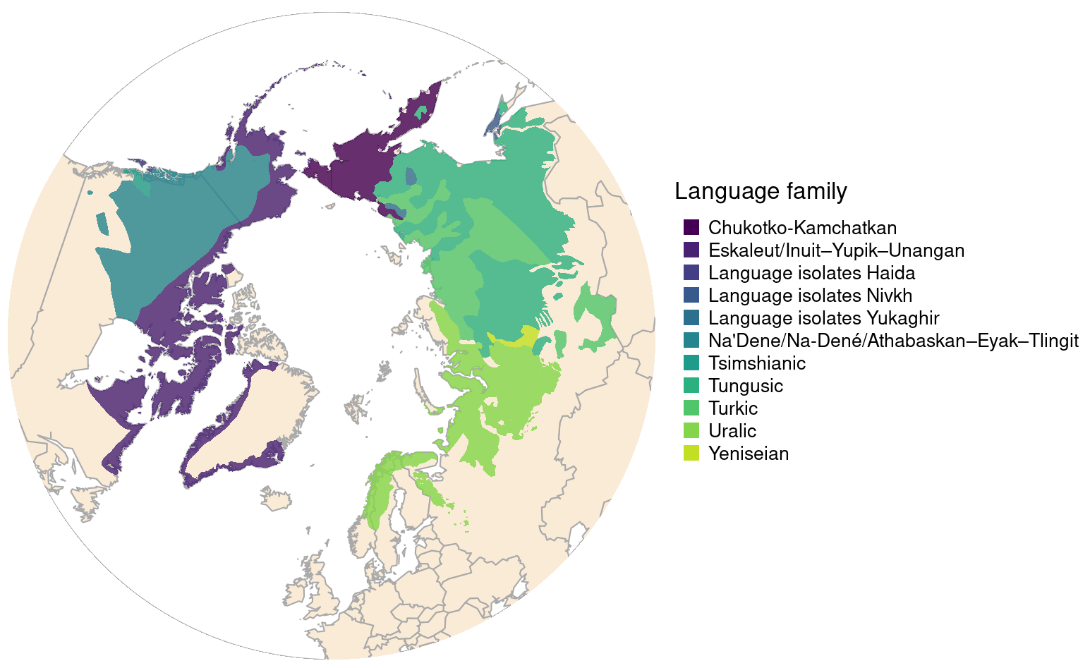
editorial (cough-cough) comment

Maybe you’re bothered by the weirdly straight polygon line in Chloe’s otherwise lovely map? Try this:

data("wrld_simpl", package = "maptools")                                                                            
w.equator <- raster::crop(wrld_simpl, extent(-180, 180, 0, 90))  %>%
  st_as_sf(coords = c("long", "lat"), crs = 4326) %>%
  st_transform(st_crs(3995))                                                               

donut <- list(cbind(x = c(0:360, 360:0, 0), y = c(rep(45, 361), c(rep(0,361)), 45))) %>% st_polygon %>%  
    st_sfc(crs = 4326) %>% st_transform(st_crs(3995)) 

fortyfive <- cbind(x = 0:360, y = rep(45, 361)) %>% st_linestring() %>%  
    st_sfc(crs = 4326) %>% st_transform(st_crs(3995)) 

Now … put it all together

par(mar = rep(.1,4))
layout(matrix(1:2, ncol =2), widths = c(1.5,1)) 

plot(fortyfive, col = "darkgrey")
plot(st_geometry(w.equator), col = "antiquewhite", add = TRUE, border = "darkgrey")
plot(donut, add = TRUE, col = "white", border = NA)
plot(lang["LangFamily"], lwd = 1, lty = 1, pal = alpha(cols, .8), add = TRUE, border = NA)

par(mar = c(0,0,6,0), xpd = NA); plot.new()
mtext(side = 3, "Language family", font = 1, line = 0, adj = 0)
legend(x = "topleft", ncol = 1, cex = 0.8, legend = labs, col = cols, pch=15, pt.cex = 1.5, bty = "n")

Do that in ggplot!