5 Spatial data in R
Data types, projections, tools
In this chapter, we discuss spatial data and examples of how to work with it in R. As with all code-dependent material, new packages and methods are constantly evolving for working with spatial data in R. We introduce current popular packages for spatial data manipulation in R, with this caveat.
5.1 What is spatial data?
Spatial data is simply data with locational information. It has both spatial attributes (e.g., geographic location) and non-spatial attributes (e.g., descriptive information, such as id name or quantitative measurements).
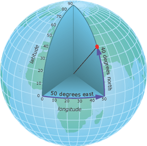
The locations of spatial data correspond to geographic coordinates that relate the data to where on Earth’s surface it occurs. These coordinates are positions on both the latitude (Y) and longitude (X) lines composing Earth’s graticular network.

So, if someone gave you a set of coordinates (longitude, latitude values), could you tell me exactly where on Earth those coordinates would be?
Probably not, because Earth is an imperfect, spinning sphere! All of those characteristics mean that the perfect spherical graticule we have for lines of latitude and longitude are not a realistic model for Earth’s true surface.

Geographic Coordinate Systems (GCS’s) are models of Earth’s surface that relate graticule (latitude, longitude) values to real locations on Earth. For example, the World Geodetic System 1984 (WGS 1984) is a GCS commonly used for mapping global data. However, their reliance on the graticule (which assumes a perfect spherical Earth) means that they are not useful for performing spatial operations where you need to understand the distance between locations.
For quantitative spatial operations, you instead want to use a Projected Coordinate System (PCS), which essentially flattens a GCS to create a more realistic model for a particular section of the Earth you are interested in. For example, the Universal Transverse Mercator (UTM) system is a common projection that divides the globe into zones. You can transform your spatial data to this projection once you figure out which zone it belongs in, allowing you to perform quantitative spatial operations on your data!

Using a GCS or PCS depends on what questions you are trying to answer and what kind of spatial operations you wish to perform. For visual or mapping purposes, the use of a GCS is often preferred, whereas any quantitative operations with spatial data generally require a transformation to a PCS. Keep in mind, the units for a GCS are in angular degrees, whereas the units for a PCS are linear measures (e.g., meters).

5.2 Types of spatial data
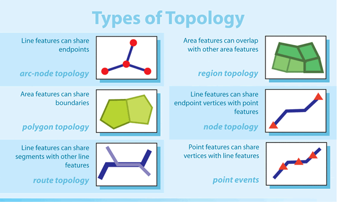
Spatial data can have a variety of characteristics, including size (e.g., length, area, perimeter), shape (e.g., point, line, polygon), and a variety of spatial relationships or topology types, including adjacency, connectivity, overlap, or proximity to other spatial objects or data.
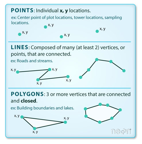
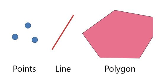
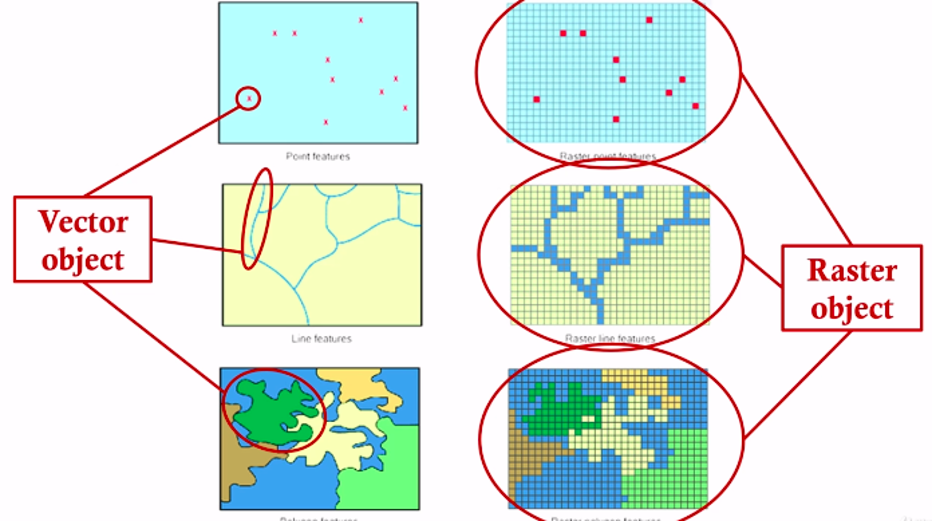
Spatial data has two broad types: vector data and raster data. Vector data is a graphical representation of “real-world” features and can come as points, lines, or polygons. This data is often stored in shapefile format (.shp).
In contrast, raster data represents data as a grid of pixels, where each pixel has a value and a resolution.
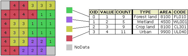
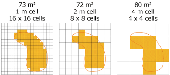
The resolution of raster data refers to the size of individual cells in the grid. If your data has a PCS, these cells will be in measurable distance units (e.g., a 1 km resolution indicates that individual cells are 1000 m x 1000 m). If your data has a GCS, resolution is referred to in angular degrees (e.g., a 0.01 degree resolution is equivalent to a ~1 km resolution).
You can cast or change your spatial data type in R. Just keep in mind that you may loose some information switching between vector to raster data (and vice versa) because of their differences in structure. Vectors have fluid boundaries, whereas rasters are composed of a bunch of little squares with sharp edges. Often, we use raster data to represent continuous data, especially from imagery, such as satellite images of abiotic data (land temperature, topography, etc). Raster data is essentially a matrix of measurable cells, making it ideal for quantitative spatial operations on layered data or any kind of matrix operations.
5.3 Importance of understanding spatial relationships for movement ecology
As discussed in previous chapters, movement data is inherently spatial. But working with movement data requires a more extensive understanding of spatial relationships and ecology than just being able to quantify and visualize the locational data for your mobile taxa of interest.
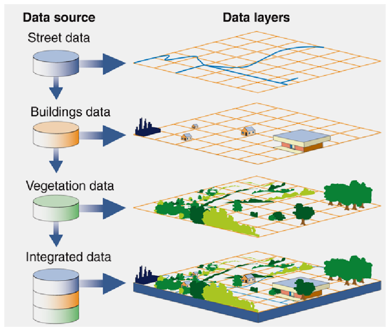
Take a minute to imagine the movement tracks of your taxa in geographic space. Most likely, your taxa exists in a spatial landscape consisting of all sorts of data, such as anthropogenic features (e.g., roads, buildings) and/or natural features (e.g., lakes, trees, topography or changes in elevation). Now, imagine these different peices of the landscape and how you would represent them as spatial data (points, lines, polygons, rasters?) and finally, how your taxa might interact with these features as they move through this landscape. These interactions are the movement-based spatial relationships you might be interested in understanding as a movement ecologist!
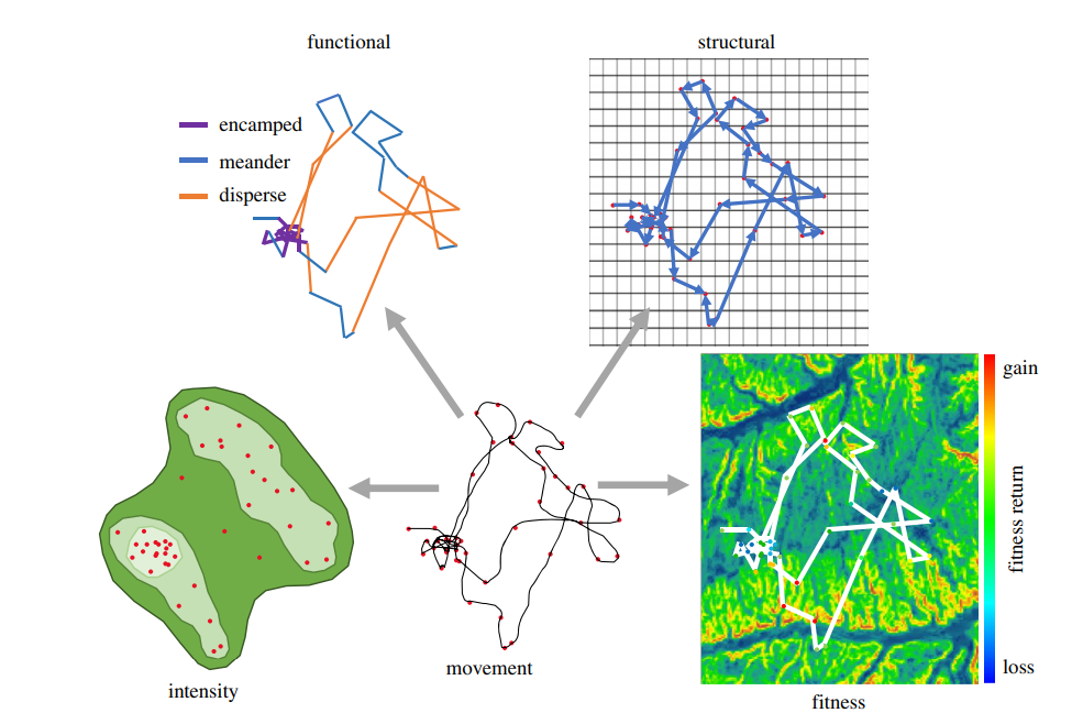
Your movement data itself can be represented and analyzed using different types of spatial data. For example, you could characterize behavior from movement data using a functional approach (e.g., represent movement states as annotated line segments), by assessing behavioral intensity (e.g., represent different levels of behavioral intensity as density isopleth polygons), by determining the structural features of a behavior (e.g., represent movement as a network of point-based behaviors), or by relating movement data locations to an underlying continuous behavioral surface (e.g., extract fitness values of locational data using a fitness or energy landscape raster) (Wittemyer, Northrup, and Bastille-Rousseau 2019-07-29, 2019-07).
5.4 Some “Tips and Tricks” for working with spatial data
The more you work with spatial data, the more you will gain your own “tips and tricks” for working with it. But here are a few essentials to start with:
You need to define the GCS and/or PCS before mapping and doing spatial operations with it. Be sure the GCS or PCS you define matches the metadata or description of the data (when in doubt, contact the owner of the data). Currently, it is easiest to define your coordinate reference system using its EPSG code.
Similarly, be sure you know the resolution and spatial extent of your raster data. Defining either your resolutions or GCS/PCS incorrectly will result in incorrect results and wonky maps!
… which is why you should always check the structure of your data before and after performing spatial operations with it. Mapping it (e.g., with an interactive mapping package such as
mapview) is a great way to check for unexpected results!When performing quantitative operations with spatial data, you should transform your data from a GCS to a PCS.
When mapping multiple layers and spatial data types (e.g., vectors and rasters), it is important that they have the same coordinate reference system and often, the same spatial extent
When doing analyses with spatial data that comes from different sources (e.g., trying to match daily locational data with environmental raster data), it is important that the spatial and temporal resolution you choose for your final product and the data layers in the analyses be logical and biologically informed. For example, if you want to match your daily locations with raster data for temperature and your taxa moves (on average) 25 km/day, does it make more sense to use temperature raster data that has a 0.01 degree (~ 1 km) resolution or that has a 1 degree (~ 100 km) resolution? Your answer is likely the latter (1 degree resolution raster), as this resolution will allow you to better match your locational data (a scale difference of 4 versus a scale difference of 25). However, you choice may also be dependent on the data available and they may not match exactly. Always go back to your research question to see if it makes sense to use these data layers together (e.g., if you expect the animal behavior from the locational data to persist ~3-4 days, this would well match the 1 degree resolution of your raster).
If you have to, you can change the spatial or temporal resolutions of your spatial data layers to better match each other (e.g. through aggregation, interpolation, averaging, or resampling) but just keep in mind that this can (and often does) cause issues with extrapolation, data degradation, and inaccuracy. Better to find data that matches well!
Keep in mind that for raster data, finer resolution data is not always better, both for the issues just mentioned AND that high resolution rasters can be massively large files that take massively long periods of time to perform spatial operations on or map. Sometimes converting your raster data to vector data (e.g., multipolgons) can speed things up.
When in doubt, Google it! There are lots of great websites, forums, books, and even groups that can help you figure out how to perform your desired spatial operations, solve error codes, etc.
5.5 R examples
We will walk through some examples in R below using recent packages for spatial data analyses and analyses. These examples are just an introduction to the many different spatial operations you can perform in R{^index-1]. There are many helpful resources out there to help with further spatial data analysis and ecology questions. This, for example, is an excellent resource: Using Spatial Data with R.
For this tutorial, we will use the following R packages: - dplyr and magrittr for data processing and manipulation, - sf and raster for loading spatial and raster data - ggplot2, mapview, ggspatial, basemaps and mapdata for mapping and visualization. - fasterize and geosphere for a few higher-level operations.
Be sure all of these have been installed.
5.5.1 Load your data
We will use two example datasets, one on sperm whales (a public Movebank dataset, study link here, originally published by Irvine et al 2017) and one on the calving grounds of Western Arctic caribou (originally published by Couriot et al 2023).
We will load our sperm whale data, stored on Excel csv files, using the “read.csv” function, and our caribou data, stored as shapefiles, using the “st_read” function from the “sf” R package. We will also bring in interesting environmental data for both, including a stack of rasters for daily sea surface temperature for the sperm whales, stored as an Rda object, and a river shapefile for the caribou.
We additionally define the CRS (coordinate reference system) of each shapefile as we read it in, using the “st_set_crs” function. We do this using their EPSG code (here, 4326 = WGS 1984 GCS) and then we transform each of them to a PCS using the sf::st_transform() function. We will walk through more examples of this shortly.
## sperm whale tracking data (Movebank)
sperm_whales <- read.csv("./data/SpermWhale_dataset.csv")
str(sperm_whales)
'data.frame': 1220 obs. of 4 variables:
$ timestamp : chr "4/3/2007 4:36" "3/27/2007 22:17" "3/28/2007 1:19" "3/28/2007 7:00" ...
$ location.long : num -112 -112 -112 -112 -113 ...
$ location.lat : num 28 28.1 28.2 28.2 28.1 ...
$ individual.local.identifier: int 4400829 4400837 4400837 4400837 4400837 4400837 4400837 4400837 4400837 4400837 ...## sea surface temperature (sst, deg Celsius) raster stack data for whales
load("./data/sst_rasterdata_whales.rda")
sst_stackclass : RasterStack
dimensions : 305, 364, 111020, 23 (nrow, ncol, ncell, nlayers)
resolution : 0.01, 0.01 (x, y)
extent : -113.561, -109.921, 26.698, 29.748 (xmin, xmax, ymin, ymax)
crs : +proj=longlat +datum=WGS84 +no_defs
names : layer.1, layer.2, layer.3, layer.4, layer.5, layer.6, layer.7, layer.8, layer.9, layer.10, layer.11, layer.12, layer.13, layer.14, layer.15, ...
min values : 23.1, 22.6, 23.3, 23.1, 22.7, 23.7, 23.7, 23.7, 23.8, 23.8, 24.6, 28.4, 28.2, 28.9, 27.5, ...
max values : 32.5, 32.5, 32.0, 30.7, 31.9, 31.6, 31.6, 30.7, 31.5, 32.3, 32.4, 32.5, 32.5, 32.5, 32.5, ... ## calving ranges and river (kobuk)
# open ranges (polygons)
calving_ranges <- st_read("./data/WAH_multiannual_calving_ranges.shp") %>%
st_set_crs(4326) %>% st_transform(3857)Reading layer `WAH_multiannual_calving_ranges' from data source
`C:\Users\egurarie\teaching\movementbook\SpatialAndMovementEcologyCourse\part2_data_and_manipulations\data\WAH_multiannual_calving_ranges.shp'
using driver `ESRI Shapefile'
Simple feature collection with 2 features and 4 fields
Geometry type: POLYGON
Dimension: XY
Bounding box: xmin: -161.9217 ymin: 67.98733 xmax: -157.9179 ymax: 70.42118
Geodetic CRS: WGS 84# open river (line)
kobuk <- st_read("./data/Kobuk.shp") %>% st_set_crs(4326) %>% st_transform(3857)Reading layer `Kobuk' from data source
`C:\Users\egurarie\teaching\movementbook\SpatialAndMovementEcologyCourse\part2_data_and_manipulations\data\Kobuk.shp'
using driver `ESRI Shapefile'
Simple feature collection with 3 features and 8 fields
Geometry type: MULTILINESTRING
Dimension: XY
Bounding box: xmin: -165.0993 ymin: 66.71652 xmax: -149.5818 ymax: 67.20265
Geodetic CRS: +proj=longlat +datum=WGS84 +no_defs5.5.2 Data exploration (sperm whale tracks)
First, we will visually look at the structure of our sperm whale data, by plotting the duration of our whale tracks by the id column. We need to also define our timestamp data, however, to be in POSIX format so that R knows the timestamp column contains Data-Time data (see also the lubridate R package for more date-time functions).
# convert timestamp data to POSIXct format (you can also use lubridate for this)
sperm_whales$timestamp <- as.POSIXct(sperm_whales$timestamp, format="%m/%d/%Y %H:%M")

# make your id column a factor and change the name to something shorter:
colnames(sperm_whales)[4] <- "id"
sperm_whales$id<-as.factor(sperm_whales$id) # we have 25 different whales!


# make a quick plot of tracks over time and by id:
ggplot(data=sperm_whales,aes(x=timestamp,y=id,color=id))+ # color bars by id levels
  geom_path(size=1) +
  theme_classic() + # I like this for a nice background theme
  xlab("Time") + ylab("ID")+ # change axis names
  theme(legend.position = "none") # don't need a legend since id names are on the left already
The results show that there are 25 different whales! For example purposes, we will subset for two of these:
## looks like we have 3 separate groups of tracked whales!
## let's subset for individuals after July 1, 2008:
sperm_whales2<- sperm_whales %>%
  filter(timestamp > "2008-07-01 00:00:00")

ggplot(data=sperm_whales2,aes(x=timestamp,y=id,color=id))+ # color bars by id levels
  geom_path(size=1) +
  theme_classic() + # I like this for a nice background theme
  xlab("Time") + ylab("ID")+ # change axis names
  theme(legend.position = "none") # don't need a legend since id names are on the left already
We plot the tracks for these individuals without making them into spatial objects, using the “ggplot2” package and specifying longitude as our x-axis and latitude as our y-axis.
ggplot(data=sperm_whales2,aes(x=location.long,y=location.lat,color=id))+ # color tracks by id
  geom_path()+
  geom_point()+
  theme_classic()+
  xlab("Longitude")+ylab("Latitude")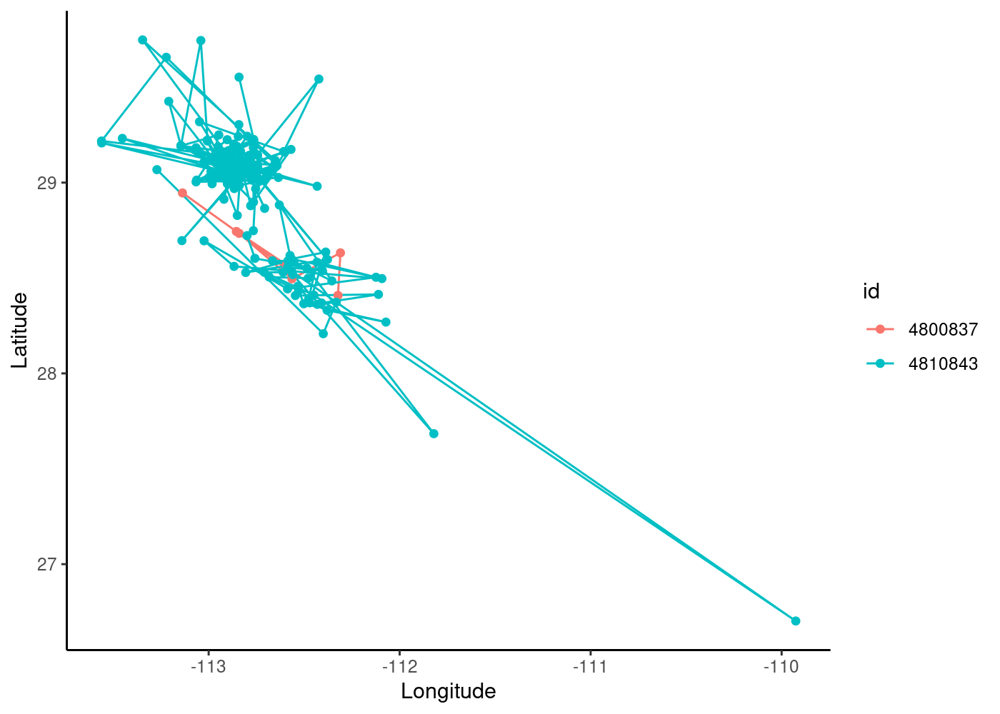
We can see that our blue individual has a lot more points in time (note also that there are likely some outlier values) and that there is spatial overlap between the individuals. We can use the facet_wrap() function in ggplot to create separate maps for each id (using “scales=free” to allow them to have different extents):
ggplot(data=sperm_whales2,aes(x=location.long,y=location.lat,color=id))+ # color tracks by id
  geom_path()+
  geom_point()+
  theme_classic()+
  xlab("Longitude")+ylab("Latitude")+
  facet_wrap(~id,scales="free")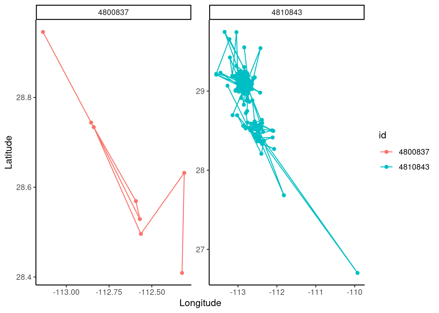
Before we make this data into a spatial object, let’s create a function to look at the median sampling frequency and temporal range for each whale track. This gives us an idea of our data resolution:
dtime <- function(t, ...) {difftime(t[-1], t[-length(t)], ...) %>% as.numeric}

data_summary <- sperm_whales2 %>%
  group_by(id) %>%
  summarize(start = min(timestamp),end = max(timestamp), MedianTimestep_hrs = round(median(dtime(timestamp, units = "hours")))) %>%
  mutate(DataSpan=round(end-start)) %>% data.frame()

data_summary
id start end MedianTimestep_hrs DataSpan
1 4800837 2008-07-02 05:03:00 2008-07-12 01:59:00 45 10 days
2 4810843 2008-07-02 00:30:00 2008-07-25 14:13:00 2 24 daysOur tracks are relatively short (10-24 days) and our first whale (ID 4800837) has a large median timestep of 45 hours! This is very typical of marine data, especially for fully pelagic species like whales, that surface unpredictably and irregularly.
5.5.3 Making our data spatial
Before we can map our whale tracks and do any spatial operations, we need to define it as a spatial object in R. This requires telling R what columns the coordinates are contained in in our dataframe and the coordinate reference system (CRS). Since our coordinates are in latitude/longitude and degrees, we will use a common GCS (WGS 1984).
# we specify the crs using the espg code
## for the GCS WGS 1984 it's 4326
sperm_whales_sf <- sperm_whales2 %>%
  st_as_sf(coords = c("location.long","location.lat"), crs=4326)
5.5.4 Plot data with the “mapview” package
Now that we have defined our data as spatial objects in R, we can create an interactive map using the “mapview” package. These maps allow you to Zoom in on your data, specify a basemap, plot different variables (similar to ggplot), and toggle specific layers on/off.
Check out this link for advanced options and examples for mapview plotting.
We are going to plot the spatial version of our whale data, using green and blue colors for the different id levels and an Esri background map.
## we use the "zcol" argument use id as our plotting variable and "col.regions" to color by the factor levels of id
## there are lots of different background map options...
mapview::mapview(sperm_whales_sf, zcol="id", col.regions=c("green","blue"),
        map.types="Esri.WorldImagery",legend=TRUE)
Looks like our whales are in the Gulf of California!
What if we want to plot the tracks instead of just the locations of the whales? We can convert the feature type from points to lines (grouped by each id) to plot the individual whale tracks:
sperm_whale_tracks <- sperm_whales_sf %>% dplyr::group_by(id) %>%
  dplyr::summarize(do_union=FALSE) %>% sf::st_cast("LINESTRING")

mapview(sperm_whale_tracks, zcol = "id", color=c("green","blue"),
        map.types="Esri.WorldImagery", legend=TRUE)
This operation is a useful one for a practical observational reason: it is good to connect points to get a sense of a track! But it is also computationally a much easier operation for mapview to draw and explore a few lines than a few thousand points.
5.5.5 Map data using the ggspatial R package
What about mapping our tracks with some interesting environmental data? A variable of interest for these whales might be sea surface temperature (sst).
Currently, the sst raster data we have (sst_stack) is a “stack” of rasters, where each raster is a layer corresponding to sst data extracted to the timestamp range and spatial extent of our whale data (source: ERDAPP/CoastWatch, NOAA Southwest Fisheries Science Center). This raster data has a temporal resolution in hours and spatial resolution of 0.01 degrees.
Raster stacks are great for performing operations on large numbers of rasters all at once. For example, if we wanted to create a raster for the mean daily sst in our region to plot beneath our tracks, we could take the mean sst across all layers in the stack:
sst_mean <- mean(sst_stack,na.rm=TRUE)

# you can plot it with base R plot functions and it automatically applies a color scale and a label:
plot(sst_mean)
plot(sperm_whales_sf, add=TRUE)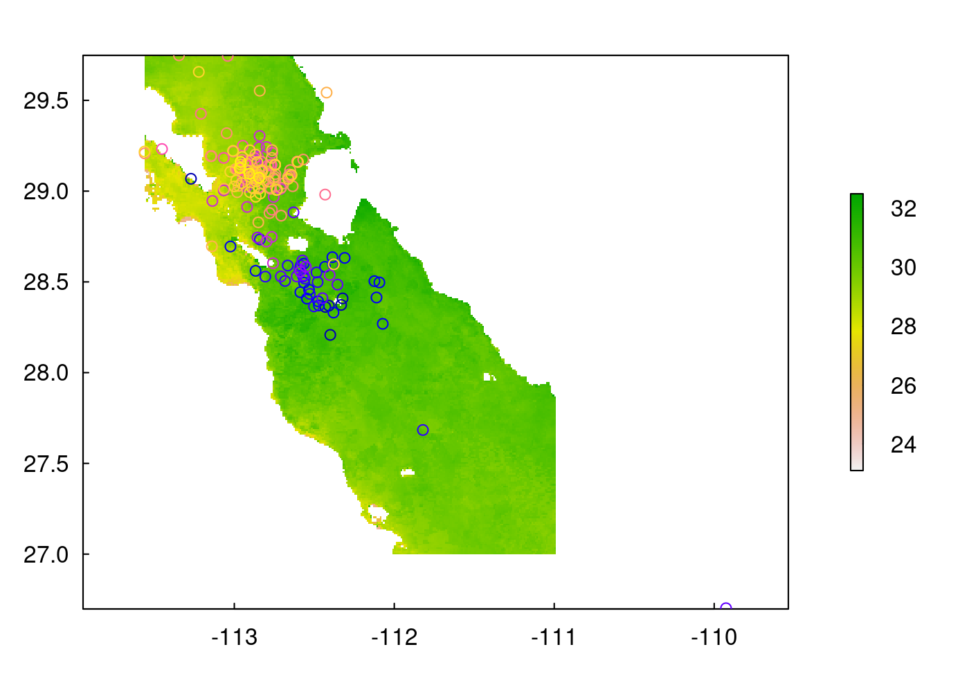
We can make some “fancier” plots of both our vector (locational points) and raster (sst) data using the ggspatial R package, which adds functions onto ggplot code. This package has access to open-source base-map tiles, as well as functions for adding a north arrow and scale bar to your maps. The zoom argument specifies the resolution of your basemap; this may take some playing with, as it is dependent on the spatial extent/resolution of your data and zooming in too much can take a very long time to plot!
Let’s start by creating a ggspatial map of just the whale tracks. We use the geom_sf() function to add our spatial whale tracks to the ggspatial map.
## the "type" argument let's you choose a basemap type (see "rosm::osm.types()" for more)
## the "zoom" argument let's you specify the number of tiles - more tiles = higher resolution but will also take longer to draw! might have to play with this a bit
library(ggspatial)

# let's plot just the tracks first:
ggplot() +
  annotation_map_tile(type = 'osm', zoom = 7) +
  annotation_scale()+
  annotation_north_arrow(height=unit(0.5,"cm"), width=unit(0.5,"cm"), pad_y = unit(1,"cm"))+
  ylab("Latitude") + xlab("Longitude")+
  geom_sf(data = sperm_whale_tracks,aes(color=id),size=1)+
  scale_color_discrete(type = c("green","blue")) +
  theme(text = element_text(size=12))
  |
  |                                                                      |   0%
  |
  |============                                                          |  17%
  |
  |=======================                                               |  33%
  |
  |===================================                                   |  50%
  |
  |===============================================                       |  67%
  |
  |==========================================================            |  83%
  |
  |======================================================================| 100%
5.5.6 Transform your data’s CRS
Generally, before performing quantitative spatial operations with our data, we need to convert our data CRS from a GCS to a PCS. To do this, you need to find a PCS that corresponds to the area your data was collected in.
Our whale data came with metadata stating that they belonged to UTM Zone 12N, so we will use this to define our PCS and transform our data, using the st_transform() function from the sf package and the corresponding EPSG code for UTM Zone 12 (32612).
Our raster data occurs in the same area, so we can also transform its CRS to the same PCS (UTM Zone 12N), but we have to use a function from the raster package, projectRaster().
# convert CRS to planar PRS
sperm_whales_sf2<- sperm_whales_sf %>%
  st_transform(4326)
Note - that projecting rasters can take a REALLY long time. As a general rule, it is smarter to
5.5.7 Make a background map using the “mapdata” package
The mapdata package has data for world-wide polygons, which we can extract, turn into a spatial objects, and crop to our study area extent. This is great if you just want a polygon of land in the background!
We use a slew of functions from the sf package to manipulate the world polygon from mapdata to something we can plot with our other data. We use the “st_cast” function to convert it from a multipolygon to polygon geometry, “st_transform” to change its CRS to a PCS, “st_crop” to crop it to the extent of our projected raster data, and then we transform it back to a GCS so that we can plot it with our whale data.
We can, again, use the ggplot2::facet_wrap() function to create separate, side-by-side maps for each unique whale id:
# extract the map data (basically, a bunch of world wide polygons
# and restrict to Mexico.

w <- map_data("worldHires",ylim = c(-90, 90), xlim = c(-180, 180)) %>%
  subset(region == "Mexico")

# make it into an sf object, change it to a polygon feature, and crop it to the spatial extent of our sst raster data
w_sf <- w %>%
  st_as_sf(coords = c("long", "lat"), crs = 4326) %>%
  group_by(group) %>%
  summarise(geometry = st_combine(geometry)) %>%
  st_cast("POLYGON") %>%
  st_crop(extent(sst_mean))

# map it with our whale track
ggplot() +
  geom_sf(data=w_sf,aes(),color="black",inherit.aes = FALSE) +
  geom_sf(data=sperm_whale_tracks,aes(color=id),size=0.7) +
  scale_color_discrete(type=c("green","blue")) +
  ylab("Latitude")+xlab("Longitude") + theme_classic() +
  theme(text=element_text(size=12),legend.position = "none") +
facet_wrap(~id) 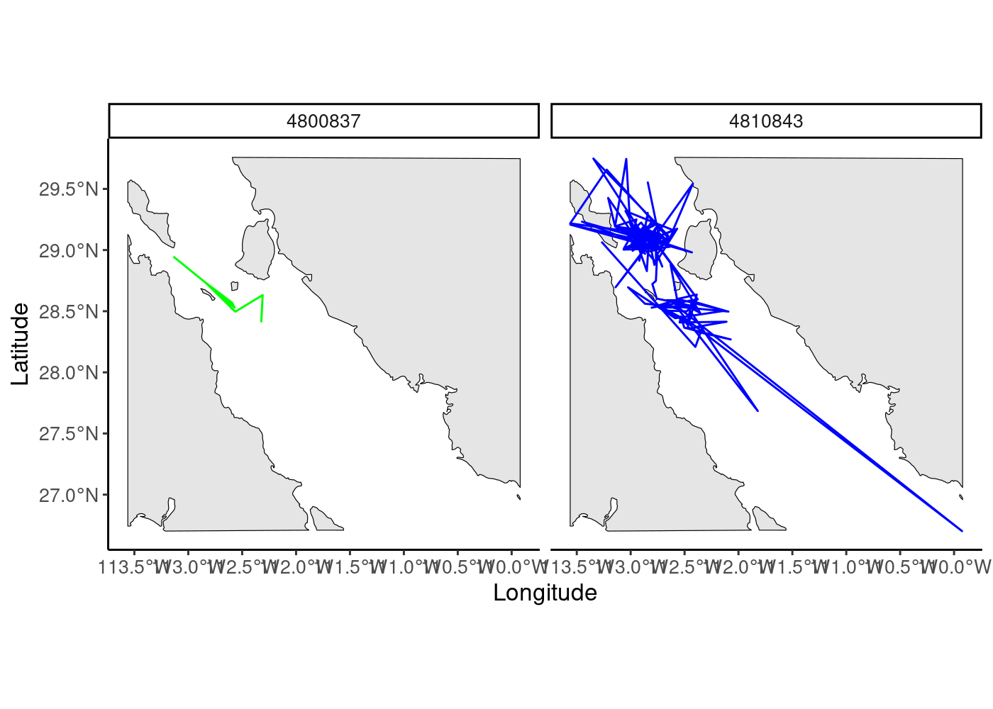
5.5.8 Map raster and vector data together
Now that the CRS of our background polygons, whale tracks, and mean sst raster all match (have the same GCS, WGS 1984), we can plot them together! Note also that our “background’ data, the sst raster and cropped world polygon, have the same spatial extent.
Before we plot our raster, we should decide how we want assign its values to color bins. If you use the base R “plot” function, it will do this automatically for you but often the bins are not as effective than if you chose them yourself.
Visualize the distribution of values in your raster data using the “hist” function:
hist(sst_mean)
We can use this distribution to decide on ~3 bins for our data. The median is close to 30 and the values range from ~ 27-32, so we define our range as 27-32 and our bin color breaks at 28, 29, 30, and 31. We use a yellow-orange-red color scheme with the function “scale_fill_gradientn”, which allows you complete control over assigning color bins to continuous data (also check out “scale_fill_gradient” and “scale_fill_gradient2”, which will bin your data into high/low or high/med/low values).
We use the “layer_spatial” function from the ggspatial R package to plot our raster data, telling ggplot that we want to fill the color values of this raster using its values (“stat(band1)”). We then define the colors to fill it with using “scale_fill_gradientn” function.
We add our whale tracks, cropped world polygon, and our whale locations, all spatial objects, using the “geom_sf” function from the sf package and assign color values to the locations using the “scale_color_discrete” function.
Finally, we facet by our different id levels to create side by side maps. Note here that the order you add your layers onto the ggplot code matters. So, here we want our raster data on the bottom, followed by our world polygon, whale tracks, and whale locations, in that order (whale locations are on “top”).
## the "layer_spatial" function allows you to plot raster data
## this time, we also plot the whale location points over the trajectories
whale_maps<-ggplot() +
  layer_spatial(data = sst_mean, aes(fill = stat(band1))) +
  geom_sf(data=w_sf,aes(),color="black",inherit.aes = FALSE)+
  geom_sf(data=sperm_whale_tracks,aes(),size=0.7,color="grey")+
  geom_sf(data=sperm_whales_sf,aes(color=id),size=1)+
  scale_color_discrete(type=c("green","blue"))+
  ylab("Latitude")+xlab("Longitude")+ theme_classic()+
  # the function below allows you to manually adjust the raster bin values, colors, and legend title
  scale_fill_gradientn("Mean SST (deg C)",colours = c("yellow","orange","red"),
                       na.value = NA,limits=c(27,32),
                       breaks=c(28,29,30,31))+
  theme(text=element_text(size=12))+
  facet_wrap(~id)

whale_maps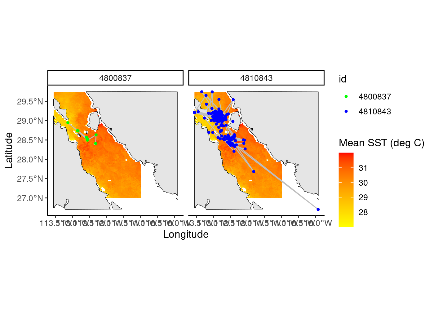
5.5.9 Export your map
Now that you have created this beautiful map, you likely want to save it somewhere. We can export images/plots/maps from R into a variety of formats (tiff, png, jpeg…) and specify both the size and quality of these images.
We will export our map to a jpeg with a 300 dpi (high) resolution and 6x3 inches size:
5.5.10 Combining vector polygons and raster basemaps
We will now demonstrate another R package you can use to map raster and vector data together, the basemaps package. This package, similar to ggspatial, allows you to grab interesting, open-source basemaps (such as rasters) for your data. You can change the map resolution using the map_res argument.
For this, we will plot our caribou calving range data (polygon) with our Kobuk river shapefile (line vector). First, we create a bounding box for our data, which defines the spatial boundaries of our map. We then extract our basemap to this bounding box, specify the map type (“topographic”), and plot this raster base map with our vector data. We use the function plotRGB() to plot our background map, a topographic raster. This function creates a red-blue-green (3 base colors) plot, a great function for raster data based on color images (e.g, Landsat data).
To add our vector data, we first grab only the geometry values of each vector, using the st_geometry() function from the sf package.
# create a "bbox" or spatial plotting limits for your map
ext <- data.frame(x = c(-170, -148), y = c(65, 72)) %>%
  st_as_sf(coords=c("x","y"), crs = 4326) %>%
  st_transform(3857) %>%
  st_bbox

# a different mapping package and function, also using the open-source osm tiles
# download the basemap
map <- basemap_raster(ext, map_service = "osm", map_type="topographic",map_res=0.3)
Loading basemap 'topographic' from map service 'osm'...# plot
plotRGB(map) # function to plot rasters with color images (e.g. Landsat data)
plot(st_geometry(kobuk), add=TRUE)
plot(st_geometry(calving_ranges)[2], add = TRUE, col = alpha("darkblue", .5))
plot(st_geometry(calving_ranges)[1], add = TRUE, col = alpha("purple", .5))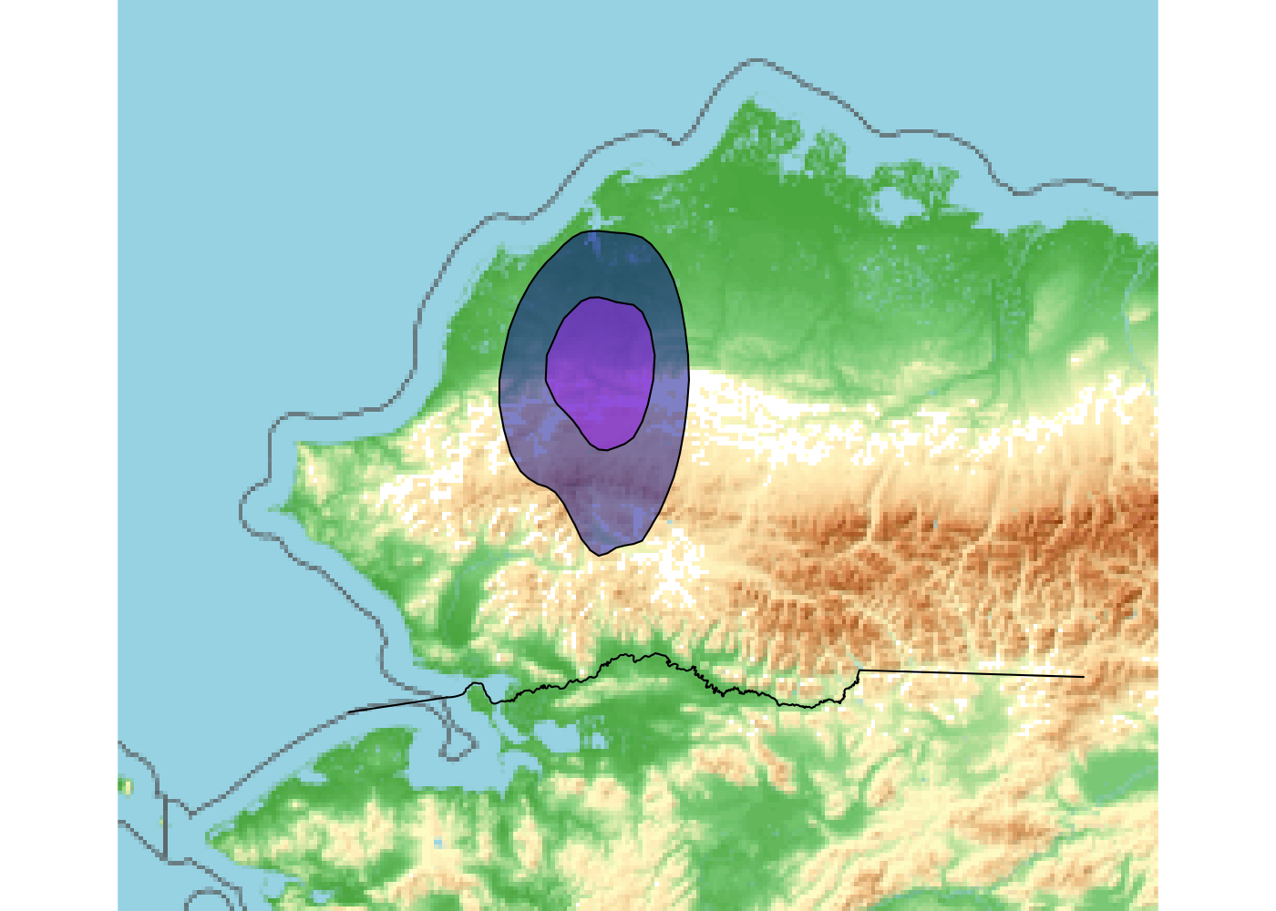
We can create an additional, interactive map of this data using the mapview package again. This time, we specify to use the ESRI shaded relief (topographic) background map:
mapview(calving_ranges,map.types = c("Esri.WorldShadedRelief"),alpha.regions=0.2,col.regions="orange")+
mapview(kobuk,col.regions="blue")
5.5.11 Spatial operations and manipulations
In the next sub-sections, we will demonstrate some examples of how to do spatial operations and manipulations with your spatial data in R.
5.5.11.1 Buffering data (st_buffer)
There are many reasons why you may want to create a buffer around your points. Below, we demonstrate how to create a 5000 m (5 km) buffer around your projected whale data, using the st_buffer() function. We visualize the results using an interactive map through mapview:
# first transform to PRG
sperm_whales_sf_2<- sperm_whales_sf %>% st_transform(32612)

# put 5 km buffer around points
sperm_whales_buff <-sperm_whales_sf_2 %>% st_buffer(5000)

# look at str
sperm_whales_buff
Simple feature collection with 191 features and 2 fields
Geometry type: POLYGON
Dimension: XY
Bounding box: xmin: 246040.3 ymin: 2948880 xmax: 611840.3 ymax: 3298168
Projected CRS: WGS 84 / UTM zone 12N
First 10 features:
timestamp id geometry
1 2008-07-02 05:03:00 4800837 POLYGON ((375407.4 3143223,...
2 2008-07-04 02:49:00 4800837 POLYGON ((376950.7 3167917,...
3 2008-07-04 04:51:00 4800837 POLYGON ((351923 3153146, 3...
4 2008-07-06 01:22:00 4800837 POLYGON ((325310.5 3179903,...
5 2008-07-06 05:44:00 4800837 POLYGON ((351383.5 3156810,...
6 2008-07-08 08:26:00 4800837 POLYGON ((349191.7 3161272,...
7 2008-07-10 03:59:00 4800837 POLYGON ((323862.6 3181034,...
8 2008-07-12 01:59:00 4800837 POLYGON ((296722.4 3203883,...
9 2008-07-02 00:30:00 4810843 POLYGON ((283918.9 3217649,...
10 2008-07-02 03:27:00 4810843 POLYGON ((367606.1 3121037,...# plot it and zoom in!
mapview(sperm_whales_buff,alpha.regions=0.1,col.regions="red")+
mapview(sperm_whales_sf_2,col.regions="blue")
5.5.11.2 Combine polygons (st_union)
If you want all of the buffers around the whale locations to have fluid/merged boundaries, you can unionize the individual polygons with “st_union” (also see “st_combine”), changing our individual polygons into one giant multipolygon.
sperm_whales_buff2<-sperm_whales_buff %>% st_union()

# look at the str
sperm_whales_buff2
Geometry set for 1 feature
Geometry type: MULTIPOLYGON
Dimension: XY
Bounding box: xmin: 246040.3 ymin: 2948880 xmax: 611840.3 ymax: 3298168
Projected CRS: WGS 84 / UTM zone 12N# plot it and zoom in!
mapview(sperm_whales_buff2,alpha.regions=0.1,col.regions="red") +
mapview(sperm_whales_sf_2,col.regions="blue")5.5.11.3 Convert polygons to rasters and vice versa
There are times when you may want to convert your polygon(s) into rasters or vice versa.
Before converting our sperm whale, multipolygon buffer into a raster, we need to add a column with some kind of variable (here, we make up a variable and set all values = 1). If your polygons had some kind of information associated with them (e.g., id name, other attribute) that you wanted to use to create a raster with, you could use that column instead. Rasters are grids of numbers so they need some kind of numbers to plot!
We transform our CRS back to a GCS, before creating a blank raster (“r”) and defining its extent, CRS, and resolution. We set the extent and CRS equivalent to that of our transformed whale buffer object. We specify the resolution of our raster to be equal to our sst raster data, 0.01 deg (~ 1 km). Keep in mind that the units for the resolution should be the same as your CRS… so if you are defining your raster with a GCS, the units should be in angular degrees (as here) and if you are defining it with a PCS (e.g., UTM), your units should match the units of the PCS (e.g., we would set our resolution to 1000 to be 1 km or 1000 m resolution).
We then use the handy little function “fasterize” from the “fasterize” R package to convert our sperm whale buffer to a raster, using our blank raster (“r”) as a template. If your data is either a dataframe/matrix or SpatialPoints/SpatialLines/SpatialPolygon object (instead of sf), you can use the “rasterize” function from the raster package to convert your vector data to a raster.
# first, we need to add a data frame column to our data so the function has something to "grab" onto
## also change back to CRS
sperm_whales_buff3 <- st_sf(var = 1, sperm_whales_buff2) %>%
  st_transform(4326)

# first we create a blank raster
r<-raster::raster()
extent(r)<-extent(extent(sperm_whales_buff3)) # set the extent to the same as polygons
crs(r)<-crs(sperm_whales_buff3) # set the crs the same as polygons
res(r)<-0.01 # set res to 0.01 deg (~ 1 km)

# look at the str
r
class : RasterLayer
dimensions : 314, 374, 117436 (nrow, ncol, ncell)
resolution : 0.01, 0.01 (x, y)
extent : -113.6124, -109.8724, 26.65309, 29.79309 (xmin, xmax, ymin, ymax)
crs : +proj=longlat +datum=WGS84 +no_defs # convert to a raster using "fasterize"
## you can also use the "rasterize" function for non-sf data
sperm_whales_buff_r<-fasterize(sperm_whales_buff3,r)
# look at the str
sperm_whales_buff_rclass : RasterLayer
dimensions : 314, 374, 117436 (nrow, ncol, ncell)
resolution : 0.01, 0.01 (x, y)
extent : -113.6124, -109.8724, 26.65309, 29.79309 (xmin, xmax, ymin, ymax)
crs : +proj=longlat +datum=WGS84 +no_defs
source : memory
names : layer
values : 1, 1 (min, max)# plot it!
plot(sperm_whales_buff_r)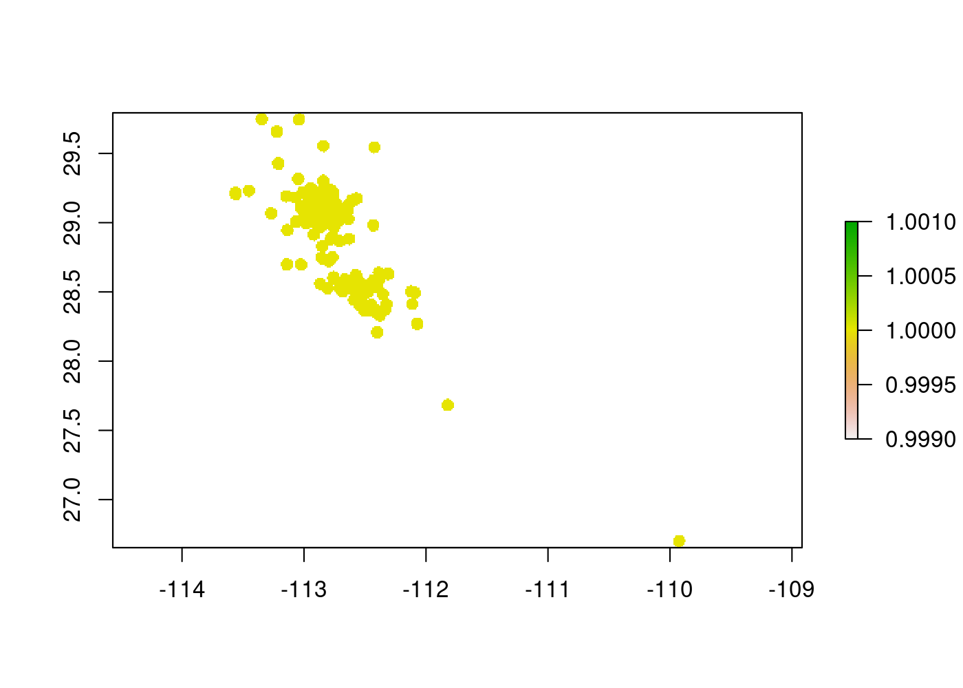
If you wanted to convert your raster back to polygons, you can use the “rasterToPolygons” function from the raster package (see also “rasterToPoints” and “rasterToContour” functions). You can specify not to include NA values in this conversion (can speed up processing time) and you can use the “dissolve=TRUE” argument to combine polygons with the same attributes to create a multipolygon.
Note here that the output is a SpatialPolygons object, not an sf object (the raster package does not work fluidly with the sf package unfortunately). Note also that the output polygon has jagged instead of smooth edges - that’s because rasters are a bunch of square cells! This issue (smooth boundaries of vectors, square edges of rasters) can have consequences when performing other spatial operations, such as extracting the values of either a raster or polygon to over-lying points, so keep this in mind.
## setting dissolve = TRUE will allow you to combine polygons with the same attributes into multi-polygons
sperm_whales_buff_poly <- rasterToPolygons(sperm_whales_buff_r, na.rm=TRUE, dissolve = TRUE)

# look at the str
sperm_whales_buff_poly
class : SpatialPolygonsDataFrame
features : 1
extent : -113.6124, -109.8724, 26.65309, 29.79309 (xmin, xmax, ymin, ymax)
crs : +proj=longlat +datum=WGS84 +no_defs
variables : 1
names : layer
value : 1 # plot it!
mapview(sperm_whales_buff_poly,col.regions="yellow")+
mapview(sperm_whales_sf,col.regions="blue")5.5.11.4 Change raster resolution
You may need to change the resolution of your raster to match another spatial layer or desired resolution. Just keep in mind that this can result in issues with extrapolation, data loss, etc!
If you want to coarsen the resolution of your raster data, you can use the raster::aggregate() function (see also the raster::resample()). Here, you specify what factor to magnify your resolution to (e.g., if we use a factor of 5 and our original resolution was 0.01 deg, our new resolution will be 0.05 deg).
If you want to do additional operations with your raster data as you aggregate it, e.g., take the mean of raster values within each new, larger cell, you can use the fun argument in this function.
## you can also use the "fun" argument to do operations with the values of cell
sperm_whales_buff_agg <- aggregate(sperm_whales_buff_r, fact=5)

# look at the str
sperm_whales_buff_agg
class : RasterLayer
dimensions : 63, 75, 4725 (nrow, ncol, ncell)
resolution : 0.05, 0.05 (x, y)
extent : -113.6124, -109.8624, 26.64309, 29.79309 (xmin, xmax, ymin, ymax)
crs : +proj=longlat +datum=WGS84 +no_defs
source : memory
names : layer
values : 1, 1 (min, max)# plot it!
plot(sperm_whales_buff_agg)
If instead you want to decrease the resolution of your raster, you can use a similar function, “disaggregate”, again specifying the factor amount to disaggregate by (e.g., if your resolution is 0.01 deg and you want to use a factor of 5, your new resolution will be 0.002 deg).
sperm_whales_buff_dagg<-disaggregate(sperm_whales_buff_r,fact=5)

# look at the str
sperm_whales_buff_dagg
class : RasterLayer
dimensions : 1570, 1870, 2935900 (nrow, ncol, ncell)
resolution : 0.002, 0.002 (x, y)
extent : -113.6124, -109.8724, 26.65309, 29.79309 (xmin, xmax, ymin, ymax)
crs : +proj=longlat +datum=WGS84 +no_defs
source : memory
names : layer
values : 1, 1 (min, max)# plot it!
plot(sperm_whales_buff_dagg)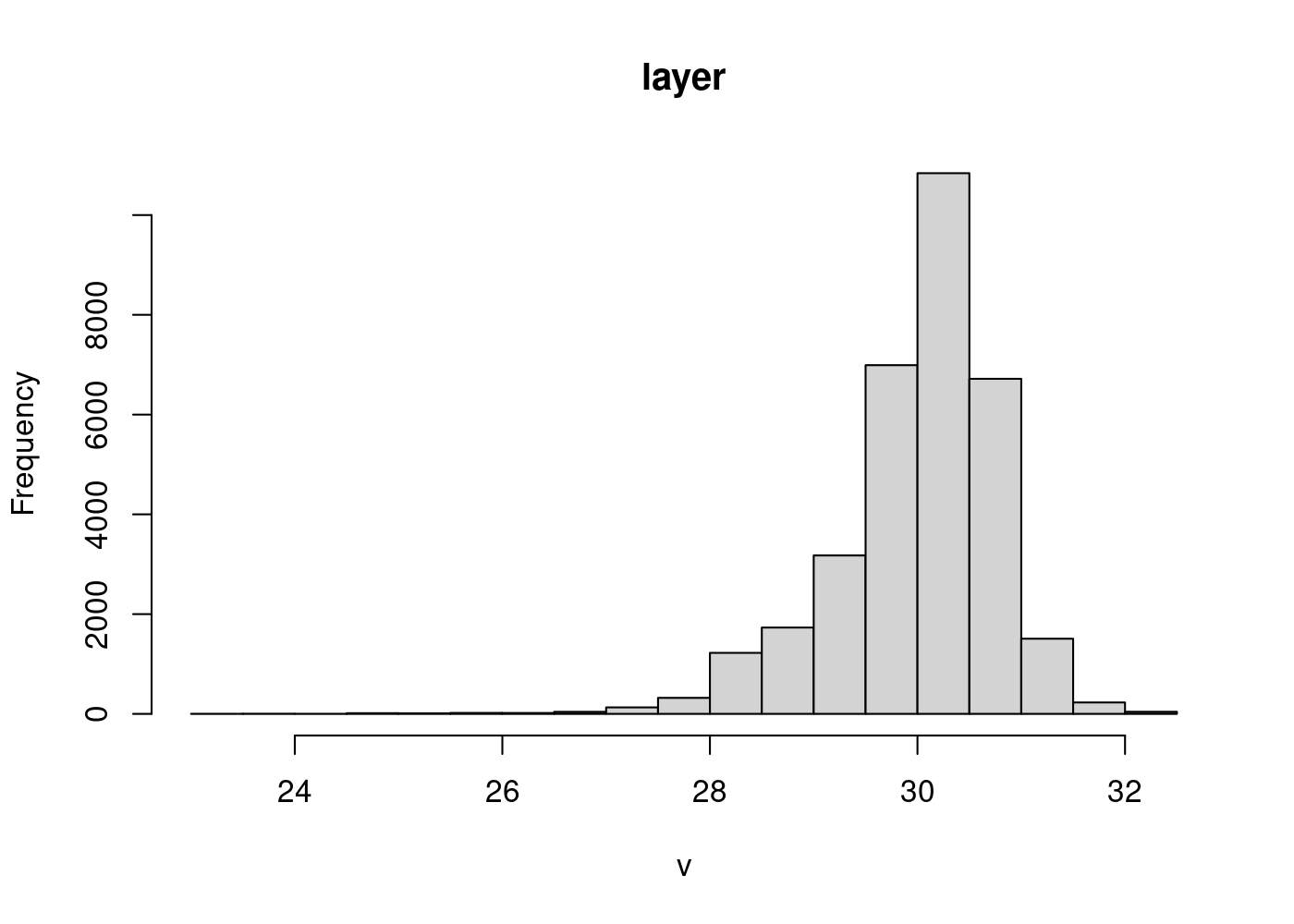
5.5.11.5 Extract values of rasters or polygons to points
If you want to extract the values of your underlying abiotic data (either vector or raster) to your locational data, you can either perform a spatial join (vector data) or you can extract values (raster data).
Spatial joins are similar to joins with non-spatial data (left join = all rows in x, (inner join = all rows in x and y, right join = all rows in y, full join = all rows in x or y).
Here, we perform a left spatial join between our projected sperm whale location data and our projected whale buffer polygon data. We then transform the CRS of the resulting object back to a GCS. Because we performed a left join, the resulting object has the same vector type as x (whale locations) but now there is an additional column (“layer”) that holds the values of the polygons overlapping in space with those locations.
# convert sp to sf
sperm_whales_buff_poly2<- sperm_whales_buff_poly %>%
  st_as_sf() %>%
  st_transform(32612)

sperm_whales_join<-st_join(sperm_whales_sf_2,sperm_whales_buff_poly2,left=TRUE) %>%
  st_transform(4326)

sperm_whales_join
Simple feature collection with 191 features and 3 fields
Geometry type: POINT
Dimension: XY
Bounding box: xmin: -113.561 ymin: 26.702 xmax: -109.926 ymax: 29.748
Geodetic CRS: WGS 84
First 10 features:
timestamp id layer geometry
1 2008-07-02 05:03:00 4800837 1 POINT (-112.323 28.409)
2 2008-07-04 02:49:00 4800837 1 POINT (-112.31 28.632)
3 2008-07-04 04:51:00 4800837 1 POINT (-112.564 28.496)
4 2008-07-06 01:22:00 4800837 1 POINT (-112.84 28.734)
5 2008-07-06 05:44:00 4800837 1 POINT (-112.57 28.529)
6 2008-07-08 08:26:00 4800837 1 POINT (-112.593 28.569)
7 2008-07-10 03:59:00 4800837 1 POINT (-112.855 28.744)
8 2008-07-12 01:59:00 4800837 1 POINT (-113.137 28.946)
9 2008-07-02 00:30:00 4810843 1 POINT (-113.271 29.068)
10 2008-07-02 03:27:00 4810843 1 POINT (-112.4 28.208)We can additionally extract underlying raster data to points, using the “extract” function from the raster package.
We can use the “extract” function with either a dataframe or an sf object. To demonstrate both, we first extract the locational information of our sperm whale points using the “st_coordinates” function from the sf package and store it as an object. We can also convert our sperm whales spatial data back to a dataframe and then add individual columns back for latitude/longitude by extracting the values from the “coords” matrix object.
We can then use the “extract” function to extract raster values to those values, using either the “coords” object or the new whale dataframe object. The resulting object is a vector, that we have to manually add back as a column to our dataframe (we can also add it to our sf data).
#extract coordinates from whale location spatial data
coords<-st_coordinates(sperm_whales_sf)

# convert spatial whale data back to data frame
sperm_whales_df<-sperm_whales_sf %>% data.frame() %>%
  mutate(lon=coords[,1],lat=coords[,2]) # add lat and long to dataframe as separate columns, grabbing them from the coords matrix (x=lon,y=lat)

# look at the str
str(sperm_whales_df)
'data.frame': 191 obs. of 5 variables:
$ timestamp: POSIXct, format: "2008-07-02 05:03:00" "2008-07-04 02:49:00" ...
$ id : Factor w/ 25 levels "4400829","4400837",..: 23 23 23 23 23 23 23 23 24 24 ...
$ geometry :sfc_POINT of length 191; first list element: 'XY' num -112.3 28.4
$ lon : num -112 -112 -113 -113 -113 ...
$ lat : num 28.4 28.6 28.5 28.7 28.5 ...# method 1: using coords
sperm_whales_extract<-extract(sperm_whales_buff_r,coords)
# look at the str
sperm_whales_extract [1] 1 1 1 1 1 1 1 1 1 1 1 1 1 1 1 1 1 1 1 1 1 1 1 1 1 1 1 1 1 1 1 1 1 1 1 1 1
[38] 1 1 1 1 1 1 1 1 1 1 1 1 1 1 1 1 1 1 1 1 1 1 1 1 1 1 1 1 1 1 1 1 1 1 1 1 1
[75] 1 1 1 1 1 1 1 1 1 1 1 1 1 1 1 1 1 1 1 1 1 1 1 1 1 1 1 1 1 1 1 1 1 1 1 1 1
[112] 1 1 1 1 1 1 1 1 1 1 1 1 1 1 1 1 1 1 1 1 1 1 1 1 1 1 1 1 1 1 1 1 1 1 1 1 1
[149] 1 1 1 1 1 1 1 1 1 1 1 1 1 1 1 1 1 1 1 1 1 1 1 1 1 1 1 1 1 1 1 1 1 1 1 1 1
[186] 1 1 1 1 1 1# can add as a column to our sperm whales df object:
sperm_whales_df$raster_values<-sperm_whales_extract
str(sperm_whales_df)'data.frame': 191 obs. of 6 variables:
$ timestamp : POSIXct, format: "2008-07-02 05:03:00" "2008-07-04 02:49:00" ...
$ id : Factor w/ 25 levels "4400829","4400837",..: 23 23 23 23 23 23 23 23 24 24 ...
$ geometry :sfc_POINT of length 191; first list element: 'XY' num -112.3 28.4
$ lon : num -112 -112 -113 -113 -113 ...
$ lat : num 28.4 28.6 28.5 28.7 28.5 ...
$ raster_values: num 1 1 1 1 1 1 1 1 1 1 ...# method 2: using sf object
sperm_whales_extract<-extract(sperm_whales_buff_r,sperm_whales_sf)
# look at the str
sperm_whales_extract [1] 1 1 1 1 1 1 1 1 1 1 1 1 1 1 1 1 1 1 1 1 1 1 1 1 1 1 1 1 1 1 1 1 1 1 1 1 1
[38] 1 1 1 1 1 1 1 1 1 1 1 1 1 1 1 1 1 1 1 1 1 1 1 1 1 1 1 1 1 1 1 1 1 1 1 1 1
[75] 1 1 1 1 1 1 1 1 1 1 1 1 1 1 1 1 1 1 1 1 1 1 1 1 1 1 1 1 1 1 1 1 1 1 1 1 1
[112] 1 1 1 1 1 1 1 1 1 1 1 1 1 1 1 1 1 1 1 1 1 1 1 1 1 1 1 1 1 1 1 1 1 1 1 1 1
[149] 1 1 1 1 1 1 1 1 1 1 1 1 1 1 1 1 1 1 1 1 1 1 1 1 1 1 1 1 1 1 1 1 1 1 1 1 1
[186] 1 1 1 1 1 1# can add as a column to our sperm whales sf object:
sperm_whales_sf$raster_values<-sperm_whales_extract
str(sperm_whales_sf)Classes 'sf' and 'data.frame': 191 obs. of 4 variables:
$ timestamp : POSIXct, format: "2008-07-02 05:03:00" "2008-07-04 02:49:00" ...
$ id : Factor w/ 25 levels "4400829","4400837",..: 23 23 23 23 23 23 23 23 24 24 ...
$ geometry :sfc_POINT of length 191; first list element: 'XY' num -112.3 28.4
$ raster_values: num 1 1 1 1 1 1 1 1 1 1 ...
- attr(*, "sf_column")= chr "geometry"
- attr(*, "agr")= Factor w/ 3 levels "constant","aggregate",..: NA NA NA
..- attr(*, "names")= chr [1:3] "timestamp" "id" "raster_values"5.5.11.6 Determine distance to an object
If you want to determine distance to an object, let’s say the distance between each of our whale spatial locations and some point, you can use the st_distance() function from the sf package. Make sure data CRS has been transformed to a PCS first!
Below, we first create a spatial point vector (27 deg lat, -111 deg long) and convert its CRS to the matching PCS of our projected whale spatial locations. We visualize where this point is with reference to our whale data using the mapview package:
# create a point with same crs
point <- data.frame(lon=-111,lat=27) %>%
  st_as_sf(coords=c("lon","lat"), crs=4326) %>%
  st_transform(32612)

mapview(point,col.regions="red")+
  mapview(sperm_whales_sf_2)
The st_distance() function returns the distance between each of our whale locations and this point, in the units of your PRS (here, meters). We can then bind this data (a vector) back to our sf data as an additional column. Note that you can use this function for other geometry types as well (points, polygons, lines…).
For some other interesting geometric operations you can perform with sf objects, also see st_area() (get the area of an sf object) and st_length() (get the length of an sf line object).
## return distance in units of PRS (meters)
sperm_whales_sf_2$dist_to_point <- st_distance(sperm_whales_sf_2,point)
str(sperm_whales_sf_2)
Classes 'sf' and 'data.frame': 191 obs. of 4 variables:
$ timestamp : POSIXct, format: "2008-07-02 05:03:00" "2008-07-04 02:49:00" ...
$ id : Factor w/ 25 levels "4400829","4400837",..: 23 23 23 23 23 23 23 23 24 24 ...
$ geometry :sfc_POINT of length 191; first list element: 'XY' num 370407 3143223
$ dist_to_point: Units: [m] num [1:191, 1] 203412 222109 226329 264042 229403 ...
- attr(*, "sf_column")= chr "geometry"
- attr(*, "agr")= Factor w/ 3 levels "constant","aggregate",..: NA NA NA
..- attr(*, "names")= chr [1:3] "timestamp" "id" "dist_to_point"An additional method you can use is with the “locator” function. You can use this function to interact with static plots (see ?locator).
For example, you can create an sf point, plot it over your sst raster, and then type “locator()” into your console. Now you can interact with your plot! Click on two locations (e.g. the red point and another spot), then hit your “Esc” button and you will get the locations of each of these points. You can then use your “st_distance” function to find the distance between these points (or you can use the geosphere package, which we will bring up next…). We include example code for this below but you will want to run this code in your console:
point<- data.frame(lon=-111,lat=27) %>%
  st_as_sf(coords=c("lon","lat"), crs=4326)

plot(sst_mean)
plot(st_geometry(point),add=TRUE,col="red")

locator()
Alternatively, you can save your click data automatically to an object (e.g., “data_click”) by preëmptively putting the number of clicks into the locator function (here, 2). After you click twice, it will automatically save your click locations into your object. We show example code for this below:
plot(sst_mean)
plot(st_geometry(point),add=TRUE,col="red")

# click twice...
data_click <- locator(2)
data_click

# convert to a sf object
data_click_sf<- data_click %>%
  data.frame() %>%
  st_as_sf(coords=c("x","y"), crs=4326) %>%
  st_transform(32612)

data_click_sf

# extract distance between points
dist<-st_distance(data_click_sf)
5.5.11.7 Spherical trigonometry with the geosphere package
If you want to perform spatial operations using spherical trigonometry and without transforming your data to a PCS, the geosphere package can be used. This package has a variety of useful functions for spatial data, including destPoint() (determine the next location given the distance and bearing or direction of travel), “bearing” (determine the direction of travel or bearing for the first location, given two successive locations), distm() (determine the distance between locations), and dist2Line() (determine the distance between points and lines or points and polygons).
For example, we can extract our whale location coordinate data using st_coordinates() and then use destPoint() to determine the location of a point that is 5000 m (5 km) and a bearing of 50 deg from each location in our data:
library(geosphere)
# extract coordinates
coords <- st_coordinates(sperm_whales_sf)

# specify bearing in degrees, distance traveled in meters
dest_point <- destPoint(coords, d=5000, b=50)

# change to a spatial object
dest_point_sf<-dest_point %>% data.frame() %>%
  st_as_sf(coords=c("lon","lat"), crs=4326)

# plot with our original points:
plot(st_geometry(sperm_whales_sf))
plot(st_geometry(dest_point_sf), add=TRUE, col="red")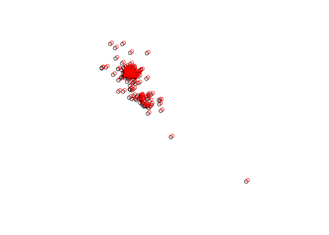
We can also use the bearing() function to determine the direction of travel between points. Note that the last location does not have a direction of travel to calculate. As such, it has an NA value at the end of the output vector.
# get the initial bearing (direction of travel, degrees) between points
dest_bearing <- bearing(coords)
str(dest_bearing)
num [1:191] 2.94 -121.18 -45.59 130.65 -26.91 ...Finally, you can use the distm() function to determine the shortest distance between points, with the default being to find this distance on the WGS1984 ellipsoid. The output has units in meters.
num [1:191, 1:191] 0 24747 25499 62096 27604 ...In the next chapter, you will learn how to manipulate and process movement data, which is inherently spatial and relies on many of the skills you just gained from this chapter.