12  Discrete time movement models

CRW origins

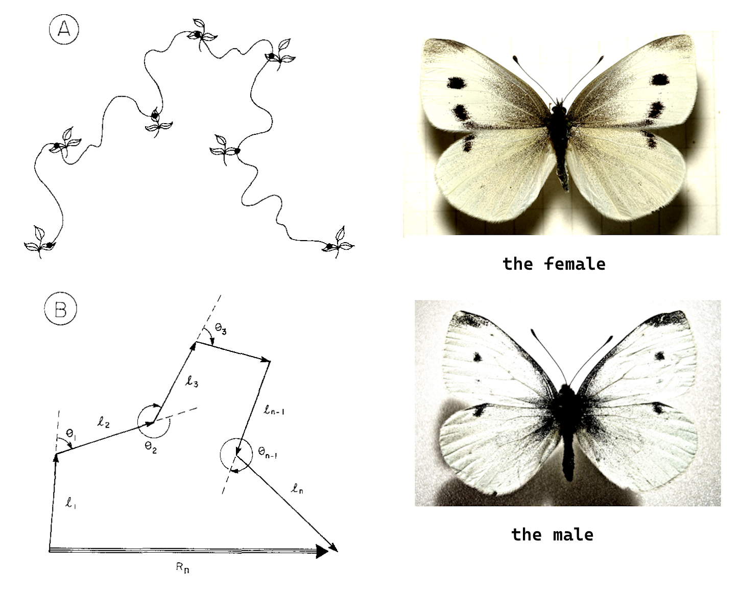
Figure 12.1: The queen of discrete movement models, the Correlated Random Walk, sketched lovingly at left from Kareiva and Shigesada (1983), based on no less lovingly following Pieris rapae - the cabbage white butterfly (at right) - flitting from flower to flower.

Goal: To understand and simulate discrete movement models including Random Walks, Autoregressive processes, Correlated Random Walks, and Multi-state Random Walks.

12.1 Introduction

Actual animal movements are invariably complex, but like any complex phenomenon, they can be thought of or reduced to some fundamental building blocks. The models are all essentially very simple, but we need to get used to the notation, the statistical properties, the very symbolic language of moving locations in space through time. To that end, we build the models hierarchically, across 1 and 2 dimensions, paying attention to the statistical properties and the parameterization of all the models, building up to the multi-state random walk - one of the real workhorses of movement analysis.

Note that notationally, we will use \(X_t\) as representing one-dimensional movement. The use of the subscript \(t\) is a clear indication that we are indexing out process in time, there is an implicit understanding that \(t \in \{0, 1, 2, 3\}\). For two-dimensional movement we will use \(\bf Z_t\), a vector containing two dimensions in \(X_t\) and \(Y_t\), or, more conveniently for many computations, as a complex number \(X_t + iY_t\).

As per usual, the emphasis is on the models - the mathematical formulations, and the statistical properties. Code can be revealed as needed. But all the basics to replicate the figures is provided here.

# only package needed - for some circular statistics

  library(circular)

# The `scantrack` function will be helpful for visualizing movements 
# in X and Y and against Time. 

  scantrack <- function(Z, cex = 0.5, ...) {
    layout(rbind(c(1,2),c(1,3)))
    plot(Z, type = "o", pch = 19, cex = cex, 
         xlab = "X", ylab = "Y", asp = 1, ...)
    points(c(Z[1], Z[length(Z)]), pch = 19, cex = 2, 
             col = c("green", "red"))
    plot(1:length(Z), Re(Z), type = "o", pch = 19, cex = cex,
         xlab = "X", ylab = "Y", ...)
    plot(1:length(Z), Im(Z), type = "o", pch = 19, cex = cex,
         xlab = "X", ylab = "Y", ...)
  }

12.2 Simple Gaussian Models

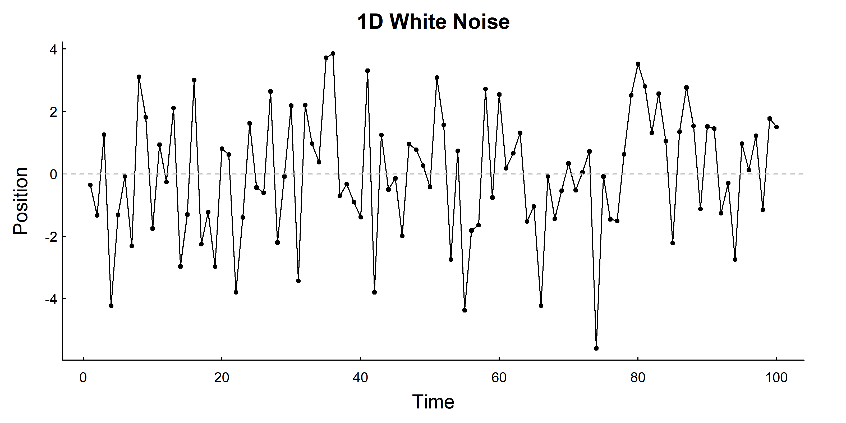
12.2.1 1D White Noise

The simplest movement model is white noise - what we might call \(WN(\sigma)\) - where each position is an independent draw from a normal distribution. We can notate that as:

\[\mathbf{X}_t \sim \sigma W_t\]

where \(W_t\) is true “white noise”, i.e. uncorrelated, independent, identical realizations of a standard normal distribution:

\[W_t \sim {\cal N}(0,1)\]

Very simple to generate:

# Parameters
sigma <- 2
n <- 100

# Simulate 1D white noise
X <- sigma * rnorm(n)

# Visualize
plot(1:length(X), X, type = "o", xlab = "Time", ylab = "Position",
     main = "1D White Noise", pch = 19, cex = 0.5)
abline(h = 0, lty = 2, col = "grey")

The properties of this model are very familiar, but we enumerate them as they are the same properties that we will be interested in comparing to more complex models. Thus:

• The expected position (or mean) \(E(X_t) = 0\), i.e. is is centered at the origin¹.
• The variance is constant: \(\text{Var}(X_t) = \sigma^2\). In the context of movement, this means that it is spatially constrained, i.e. has a one-dimensional equivalent of a “home range”).
  
• No autocorrelation: each position is completely independent

¹ It is trivial to shift the mean of this (and all subsequent) models by simply adding that new mean, e.g. $X = WN() + .

² I refuse to use the word “regression” for … reasons.

For ecologists, this process might be most familiar as the bahavior that is assumed behind the i.i.d. (independent and identically distributed) residuals of an ordinary linear model².

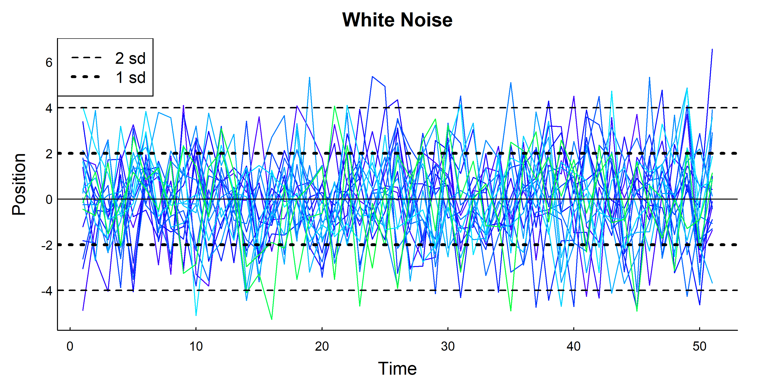
Here’s is what a white noise process looks like:

i <- 1:20; n<- 50
X <- sapply(i, function(x) rnorm(n+1, sd = sigma))
matplot(X, type = "l", lty = 1, col = topo.colors(n), xlab = "Time", 
        ylab = "Position", main = "White Noise")
abline(h = c(-2*sigma, -sigma, 0, sigma, 2*sigma), lty = c(2,3,1,3,2), col = "black", lwd = c(1.5,3,1,3,1.5))
legend("topleft", lwd = c(1.5,3), lty = c(2,3), legend = c("2 sd", "1 sd"))

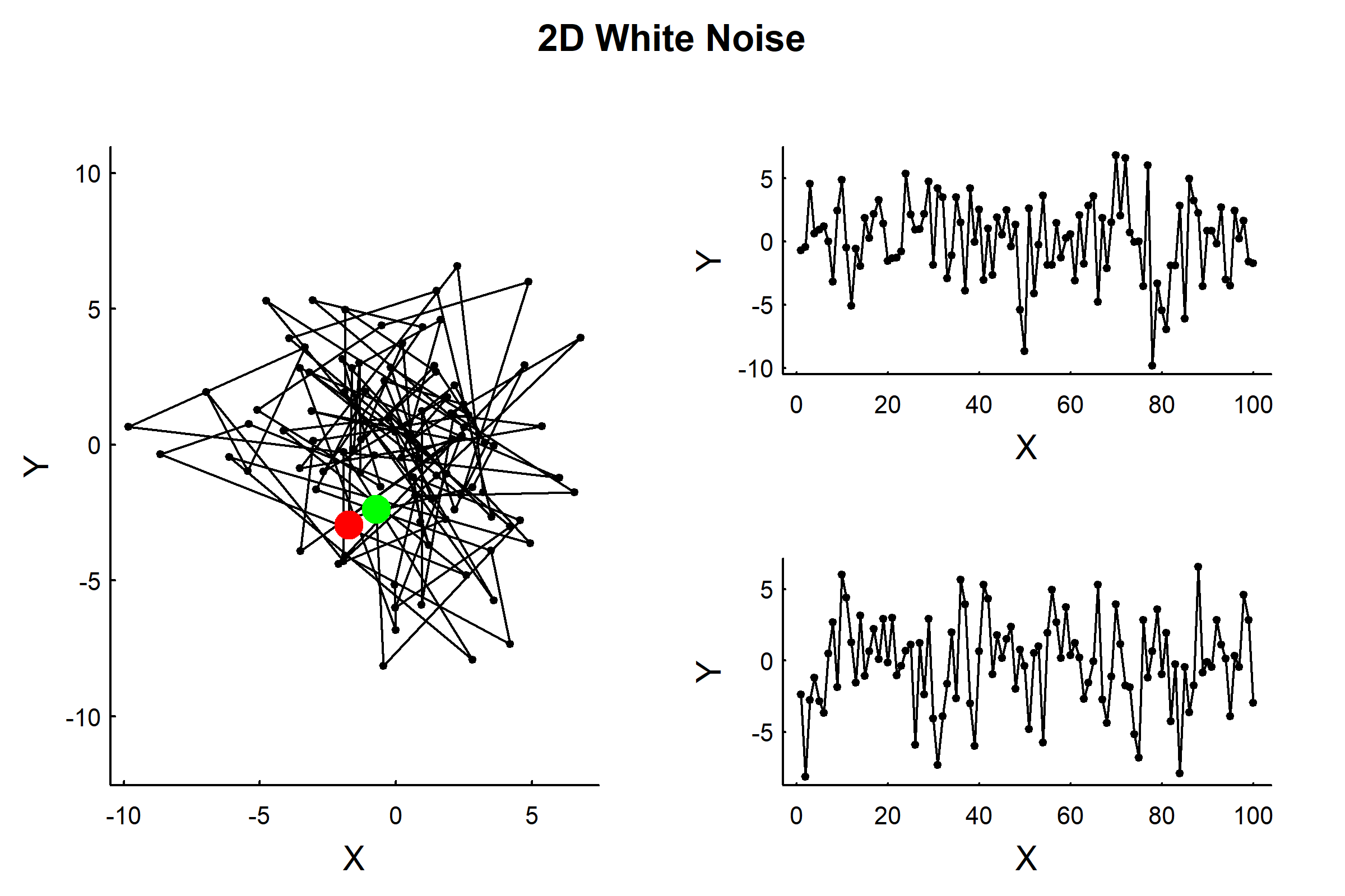
12.2.2 2D White Noise

Extending this to 2 dimensions is as simple as making X and Y each be a WN(\(\sigma\)) process. For convenience, we’ll use complex numbers, and the scantrack function to see how this process changes in time.

\[\mathbf{Z}_t \sim \mathcal{N}(0, \sigma^2)\]

# Parameters
sigma <- 3
n <- 100

# Simulate 2D white noise using complex numbers
Z <- rnorm(n, sd = sigma) + 1i * rnorm(n, sd = sigma)

# Visualize
scantrack(Z)
title("2D White Noise", outer = TRUE)

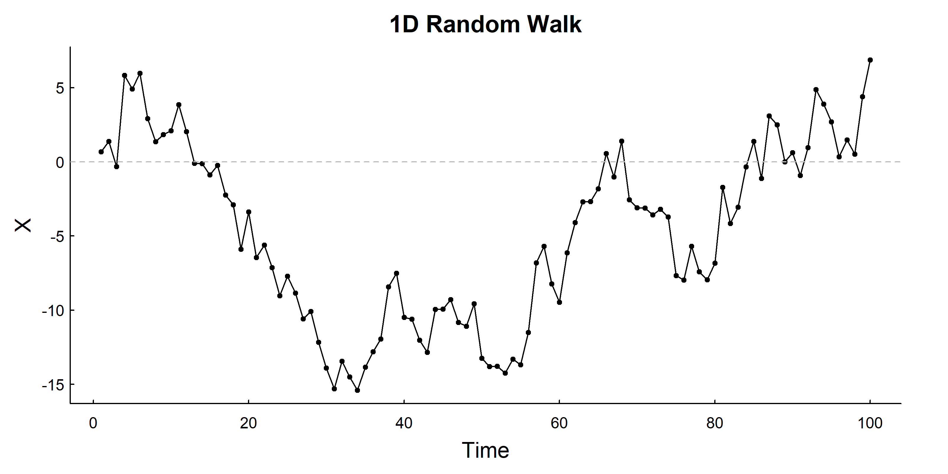
12.2.3 1D Random Walk

A random walk, in general, is a process where the location is a cumulative sum of a series of steps. The 1-dimensional random walk, where each step (not each location) is drawn from a normal distribution.
\[X_t = X_{t-1} + \sigma W_t\]

where \(W_t \sim \mathcal{N}(0,1)\) is white noise and \(\sigma\) controls step size.

# Parameters
sigma <- 2
n <- 100

# Simulate 1D random walk
X <- cumsum(rnorm(n, sd = sigma))

# Visualize
plot(1:length(X), X, type = "o", xlab = "Time",
     main = "1D Random Walk", pch = 19, cex = 0.5)
abline(h = 0, lty = 2, col = "grey")

Properties: - Expected position: \(E(X_t) = 0\) (on average stays at origin) - Variance: \(\text{Var}(X_t) = \sigma^2 t\) (variance increases with time) - Unconstrained - will wander to infinity!

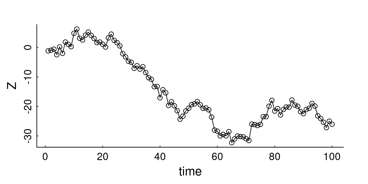
Here’s one way to visualize all the random walks, and how the standard deviation increases as the square root of time:

i <- 1:100
X <- sapply(i, function(x) c(0,cumsum(rnorm(n))))
matplot(X, type = "l", lty = 1, col = topo.colors(100), xlab = "Time", 
        main = "Random")
curve(2*sqrt(x), add = TRUE, lwd = 1.5, xlim = c(0,100))
curve(sqrt(x), add = TRUE, lwd = 3, xlim = c(0,100))
curve(-sqrt(x), add = TRUE, lwd = 3, xlim = c(0,100))
curve(-2*sqrt(x), add = TRUE, lwd = 1.5, xlim = c(0,100))
legend("topleft", lwd = c(1.5,3), legend = c("2 sd", "1 sd"))

12.2.4 2D Random Walk

We can extend this to 2 dimensions by creating independent random walks in X and Y. We’ll use complex numbers for convenient 2D representation.

\[\mathbf{Z}_t = \mathbf{Z}_{t-1} + \sigma \mathbf{W}_t\]

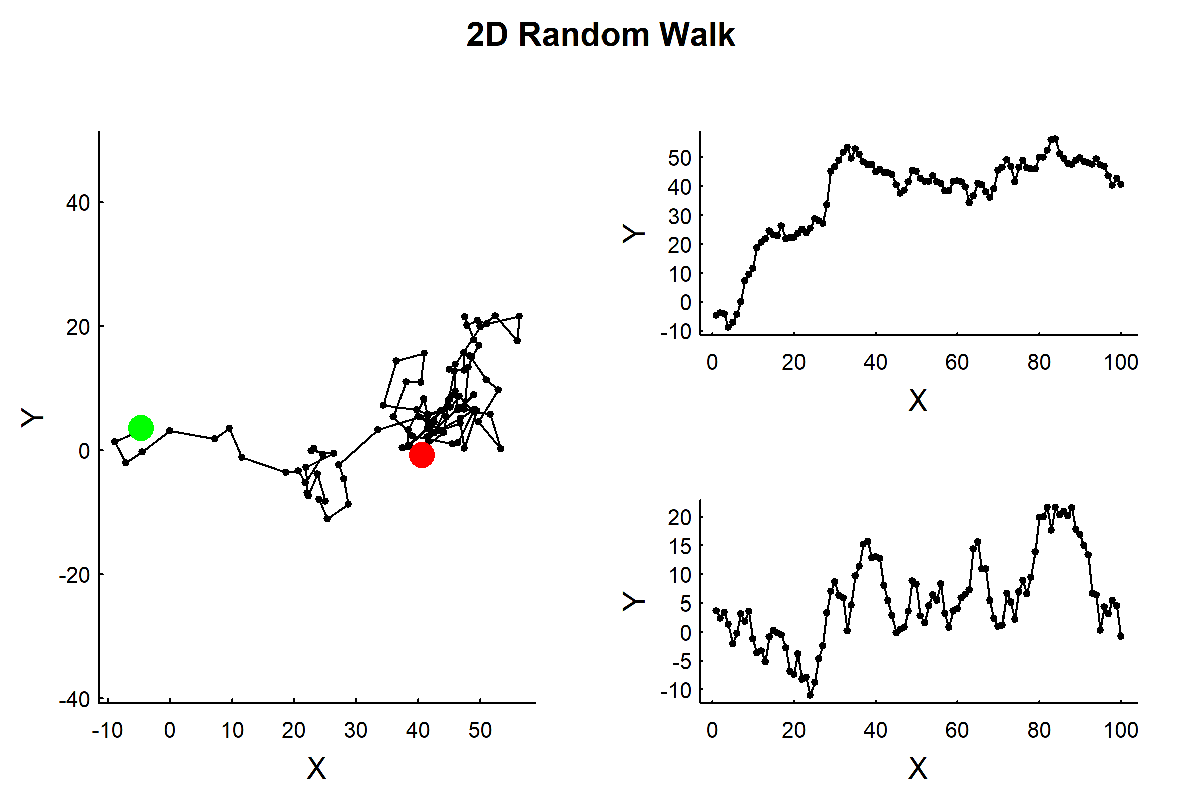
# Parameters
sigma <- 3
n <- 100

# Simulate 2D random walk using complex numbers
Z <- cumsum(rnorm(n, sd = sigma)) + 1i * cumsum(rnorm(n, sd = sigma))

# Visualize
scantrack(Z)
title("2D Random Walk", outer = TRUE)

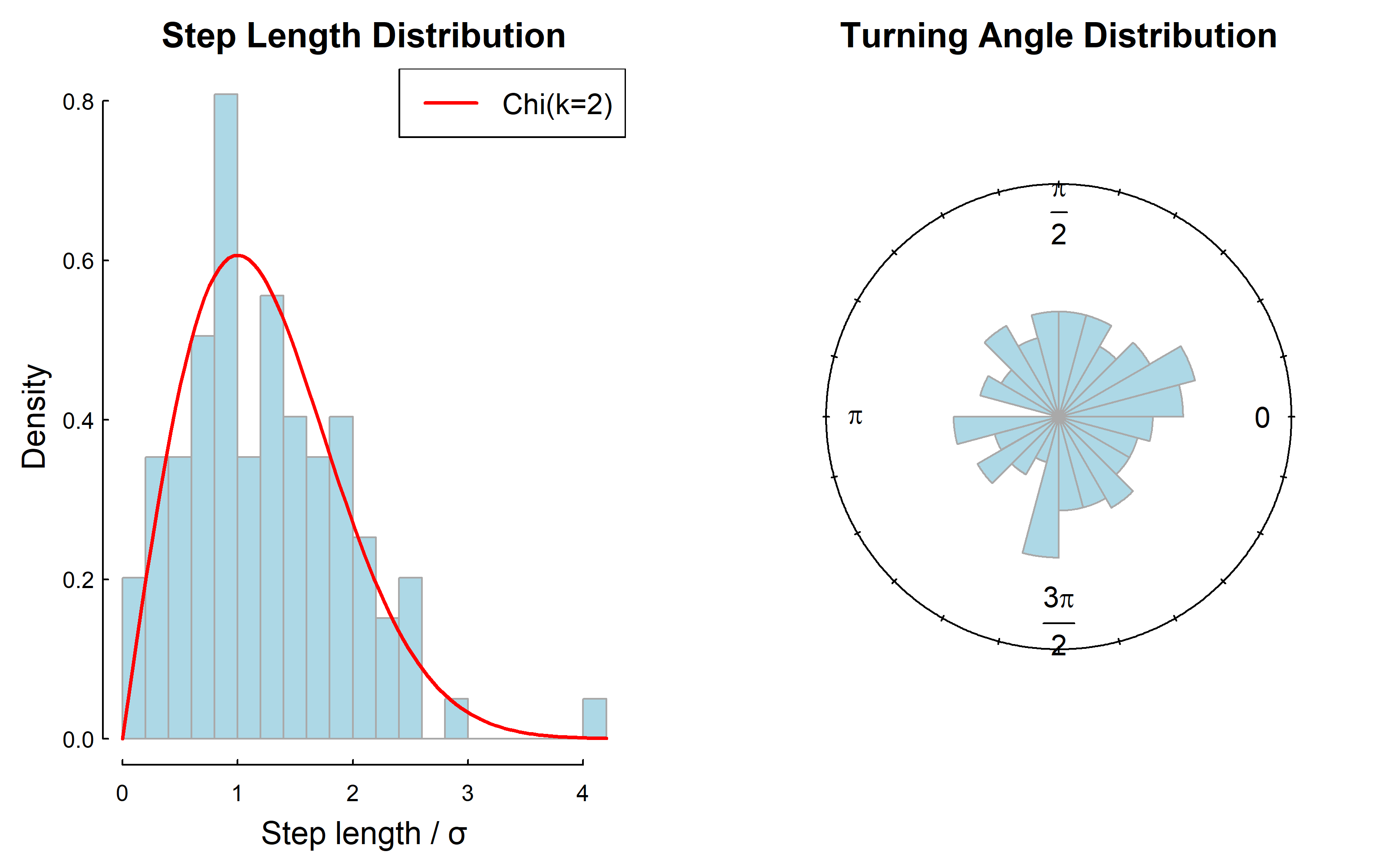
The properties of 2D Random Walk Let’s examine the step lengths and turning angles:

# Calculate steps
S <- diff(Z)
step_lengths <- Mod(S)
turning_angles <- diff(Arg(S))

# Plot step length distribution
par(mfrow = c(1, 2))
hist(step_lengths / sigma, breaks = 20, freq = FALSE, 
     main = "Step Length Distribution",
     xlab = "Step length / σ", col = "lightblue", border = "darkgrey")
curve(chi::dchi(x, df = 2), add = TRUE, col = "red", lwd = 2)
legend("topright", "Chi(k=2)", col = "red", lwd = 2)

# Plot turning angle distribution
rose.diag(turning_angles, bins = 24, prop = 2, col = "lightblue", 
          border = "darkgrey", main = "Turning Angle Distribution")

Key properties: - Turning angles are uniformly distributed: \(\theta \sim \text{Unif}(-\pi, \pi)\) - Step lengths follow a Chi distribution with k=2 - Expected step length: \(E(|S|) = \sqrt{2}\sigma\)

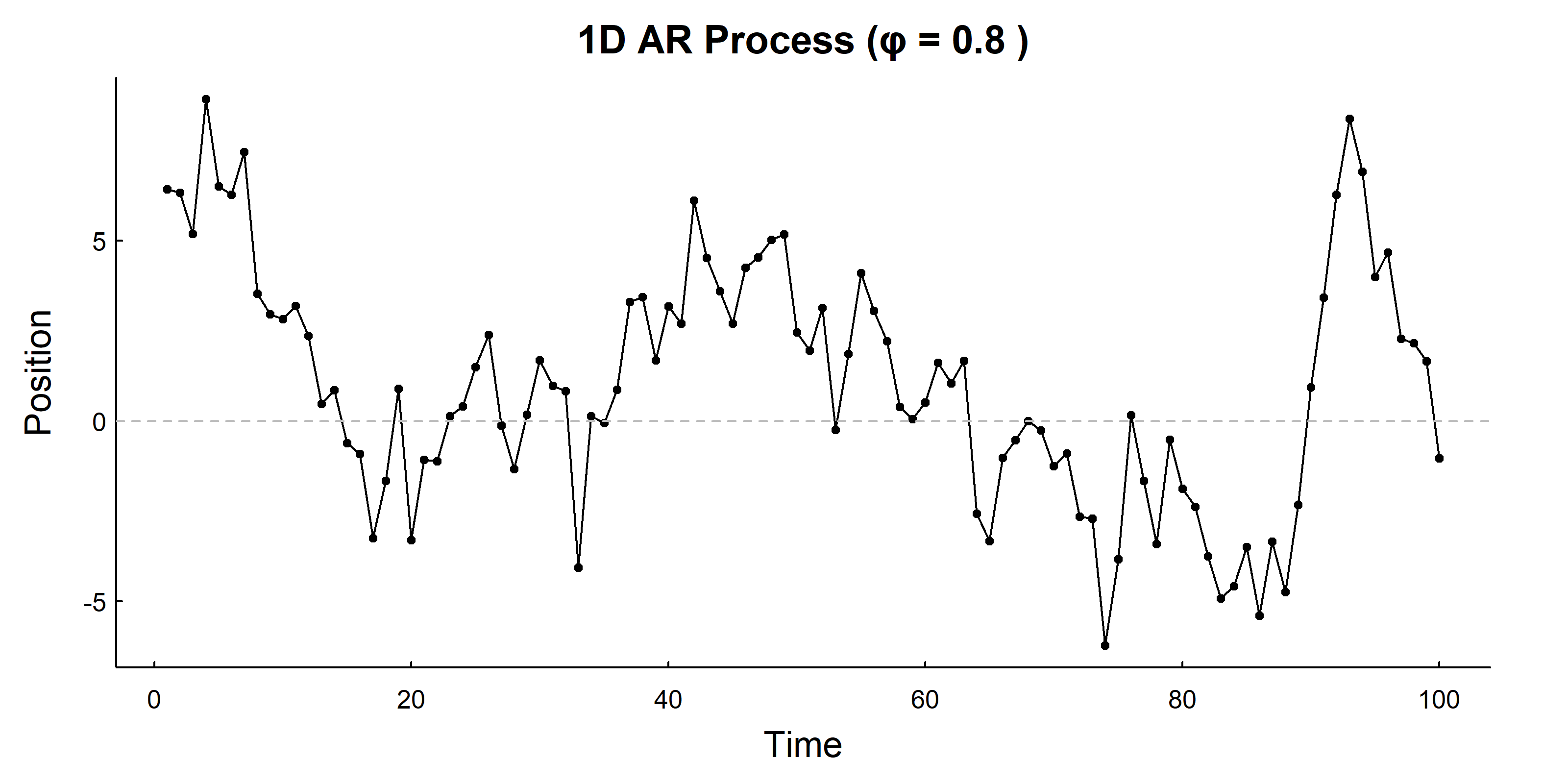
12.2.5 1D Autoregressive Process (AR)

Unlike random walks that wander to infinity, autoregressive processes are spatially constrained.

\[X_t = \phi X_{t-1} + \sigma W_t\]

where \(\phi\) is the autocorrelation parameter (0 < \(\phi\) < 1).

# Function to simulate 1D AR process
AR1D <- function(n = 100, sigma = 2, phi = 0.8, mu = 0) {
  X <- numeric(n)
  X[1] <- rnorm(1, 0, sigma)
  for(i in 2:n) {
    X[i] <- phi * X[i-1] + rnorm(1, 0, sigma)
  }
  X + mu
}

# Simulate
sigma <- 2
phi <- 0.8
n <- 100
X <- AR1D(n, sigma, phi)

# Visualize
pars()
plot(1:length(X), X, type = "o", xlab = "Time", ylab = "Position",
     main = paste("1D AR Process (φ =", phi, ")"), pch = 19, cex = 0.5)
abline(h = 0, lty = 2, col = "grey")

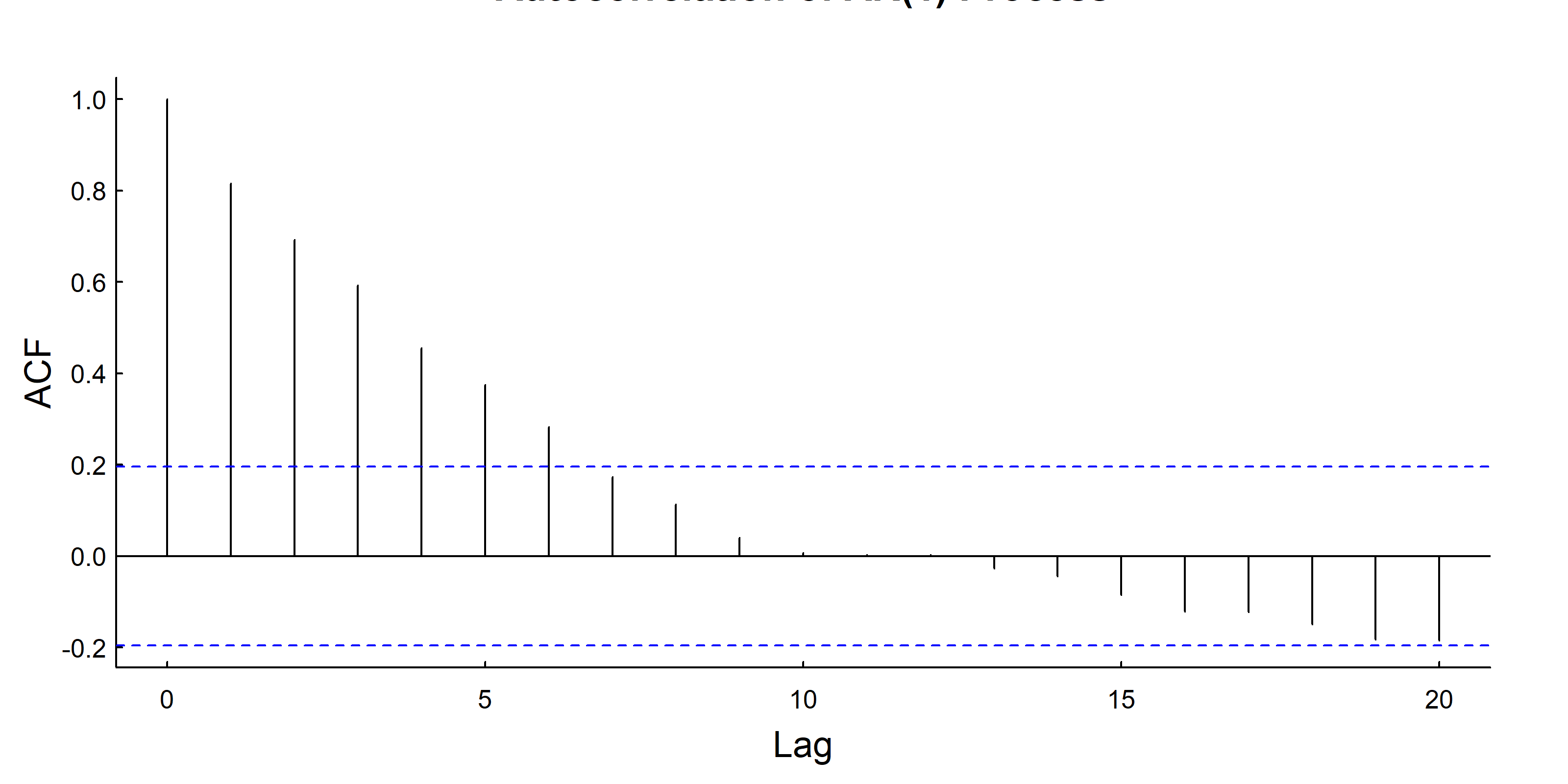
Properties: - Expected position: \(E(X_t) = 0\) (or \(\mu\) if shifted) - Variance: \(\text{Var}(X_t) = \frac{\sigma^2}{1-\phi^2}\) (spatially constrained!) - The autocorrelation parameter \(\phi\) controls how strongly positions are correlated

Let’s examine the autocorrelation:

acf(X, main = "Autocorrelation of AR(1) Process")

Notice the exponential decay in the autocorrelation function - this is characteristic of AR processes.

12.2.6 2D Autoregressive Walk

We can extend the AR process to 2D by having independent AR processes in X and Y dimensions.

\[\mathbf{Z}_t = \phi \mathbf{Z}_{t-1} + \sigma \mathbf{W}_t\]

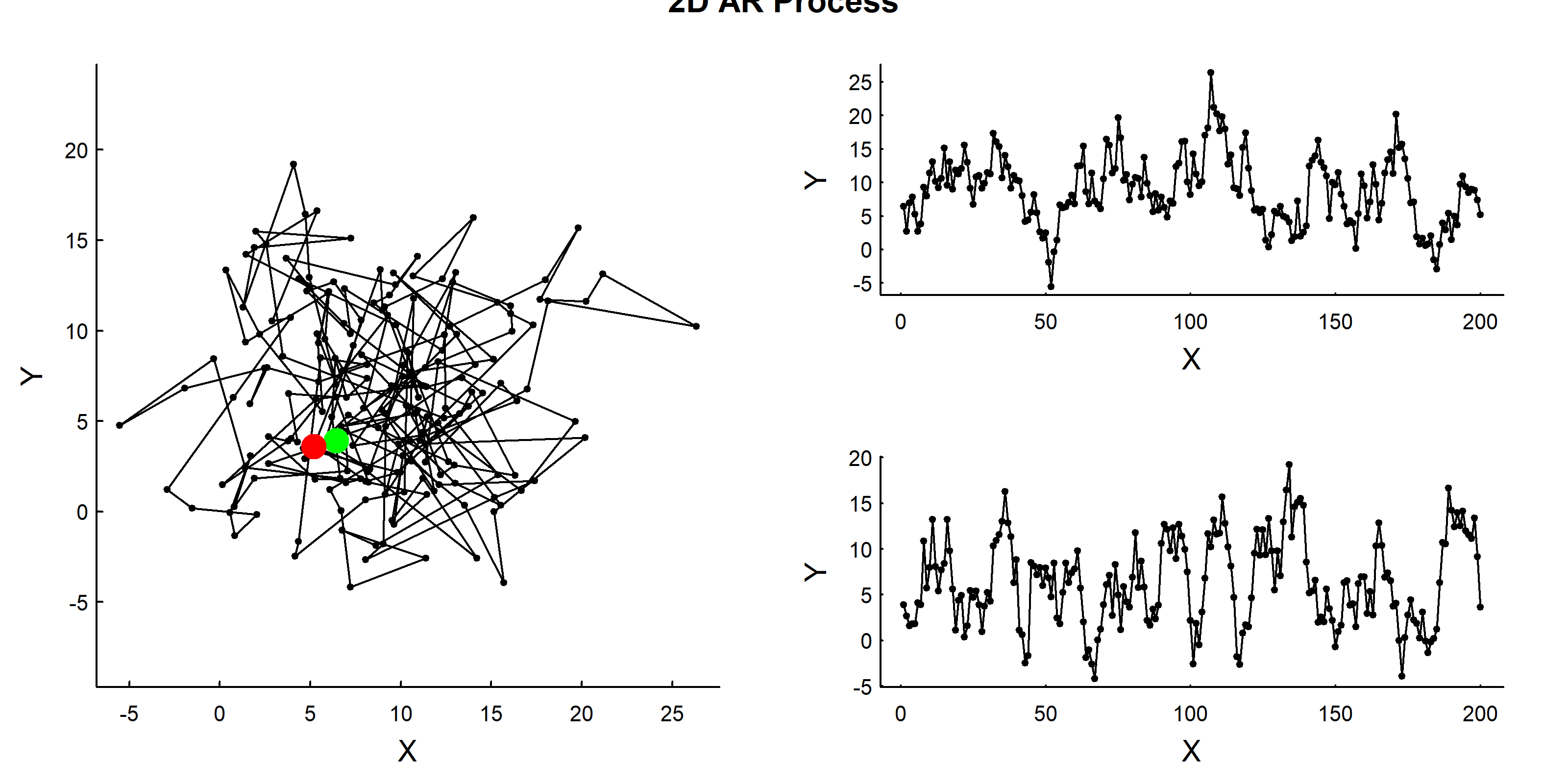
# Function to simulate 2D AR process
AR2D <- function(n = 100, phi = 0.8, sigma = 1, mu = 0) {
  X <- AR1D(n, sigma, phi, Re(mu))
  Y <- AR1D(n, sigma, phi, Im(mu))
  X + 1i * Y
}

# Simulate
Z <- AR2D(n = 200, phi = 0.8, sigma = 3, mu = 10 + 1i*5)

# Visualize
scantrack(Z)
title("2D AR Process", outer = TRUE)

This looks like (very basic) home-ranging behavior! The animal stays within a boundd area. We can compute the theoretical 95% home ranging area of this process as:

\[A \approx \frac{6\pi\sigma^2}{1-\phi^2}\]

where 6 ≈ -2 log(0.05). Thus, for example, with \(\sigma = 3\) and \(\phi = 0\) (i.e. for a white noise), the 95% ranging area is around 170, while for an autocorrelation of \(\phi = 0.8\) it leaps up to 470. More importantly, you can easily invert the parameterization of this model and define it as a \(AR_{2D}(A, \phi)\), which is then parameterized in terms of

sigma <- 3
phi <- c(0, 0.8)
-2*log(.05)*pi*sigma^2/(1-phi^2)

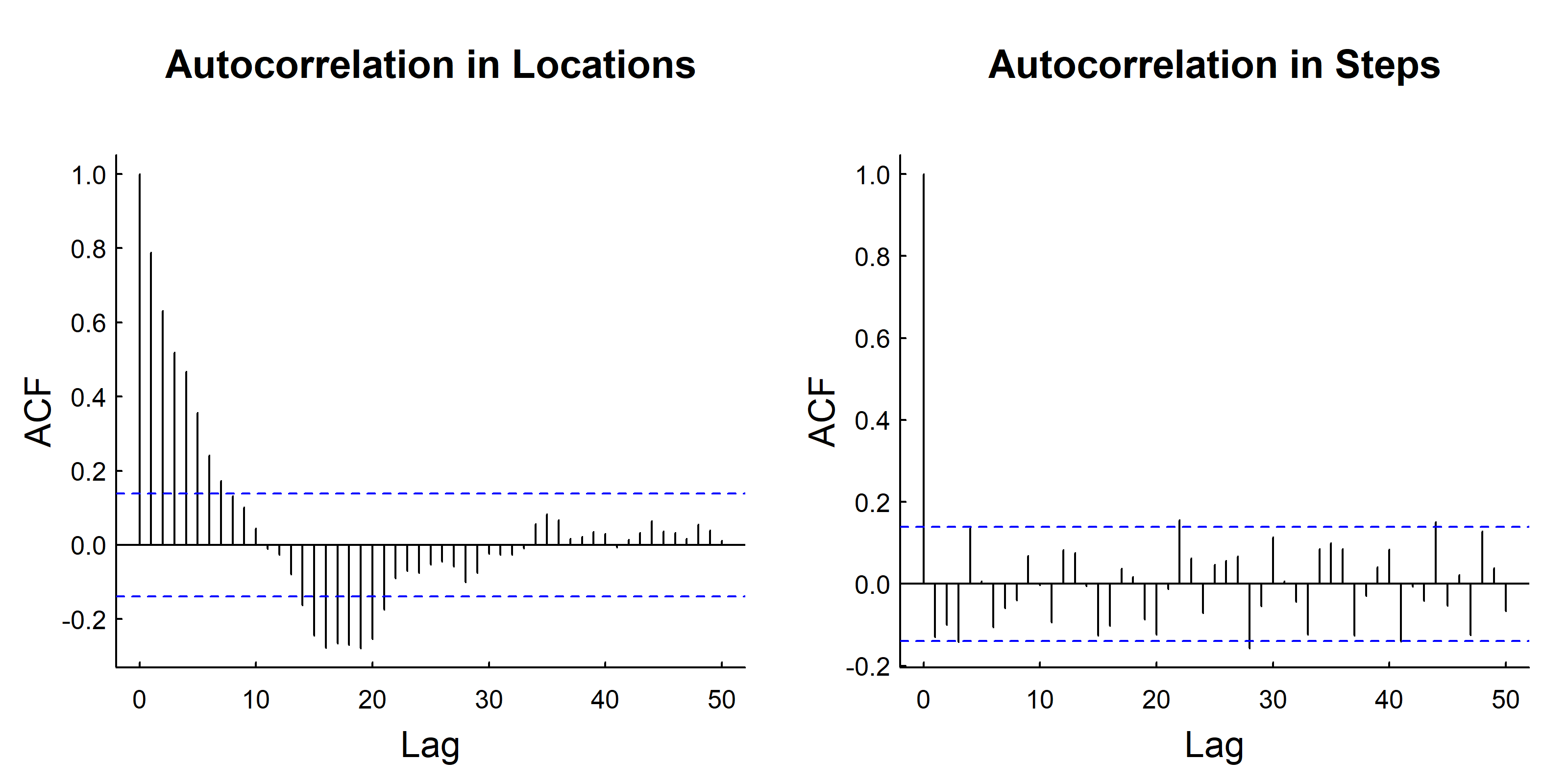
Note that The AR process is autocorrelatied in locations but NOT in the steps:

acf(Re(Z), main = "Autocorrelation in Locations", lag.max = 50)
acf(Re(diff(Z)), main = "Autocorrelation in Steps", lag.max = 50)

12.3 Correlated Random Walk (CRW)

“Correlated random walk” is the name given by Kareiva and Shigesada (1983) to a process in which discrete steps - in their case, the displacements of the cabbage white butterfly (Pieris rapae, figure Figure 12.1) between flowers, and of the pipe-vine swallowtail (Battus philenor) catterpillar crawling in a field and tagged with flags every 2 minutes. Essentially, the authors found that there is some persistence in the orientation of the discrete steps, modelled that persistence with a “clustered” turning angle distribution, and went on to analyze the rate of “diffusivity” of the resulting process.

It bears noting that while Kareiva and Shigesada (1983) coined the term and acronym CRW, and provided a nice foundataional piece of analysis to go with it, this model was studied extremely exhaustively in a pair of papers from the 1950s by Patlak (1953a), Patlak (1953b). In these largely forgotten papers the effect of various forms of correlation and anisotropy in individual movement steps are related to diffusion approximations, with explicit derivations of expected displacements and rigorous tests for external orientation. Patlak considers a discretization of movement that consists of step lengths l, the turning angles \(\theta\) and time intervals \(t\) drawn from some arbitrary distributions and predicted the displacements and theoretical rates of diffusion for such movers in terms of the mean and variance or step lengths, the mean cosine of turning angles, and the mean time interval. The analysis was exhaustive, but too far ahead of the data to be applied in any meaningful way.

\[Z_t = Z_{t-1} + S_t\]

• \(\theta = \text{Arg}(S) \sim \text{some distribution}\)
• \(|S| \sim \text{some distribution}\)

In a Correlated Random Walk, turning angles are autocorrelated, creating directional persistence.

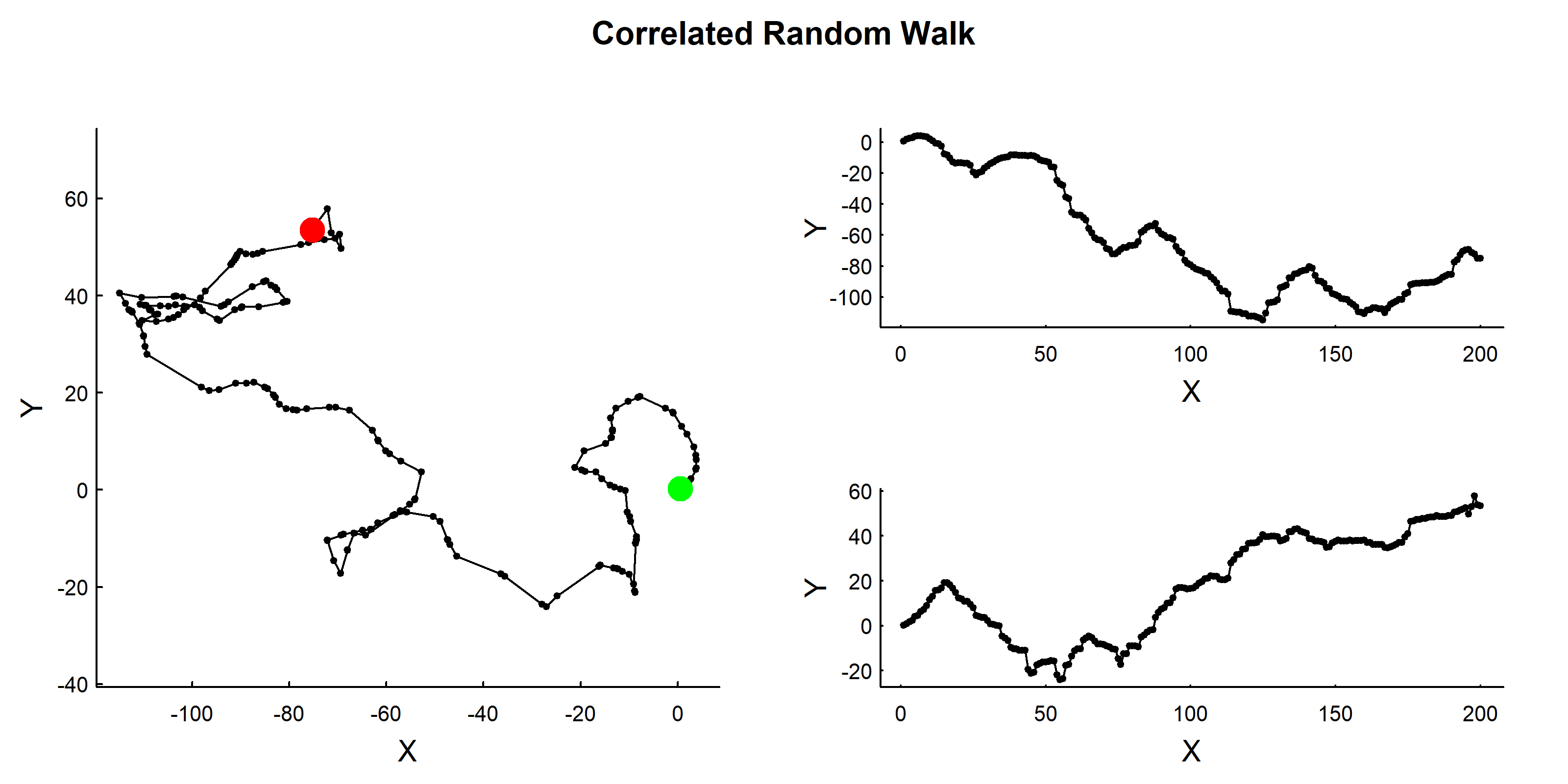
# Function to simulate CRW
CRW <- function(n = 100, rho = 0.8, alpha = 1, beta = 2) {
  # rho: concentration parameter for wrapped Cauchy (0 = uniform, 1 = no turning)
  # alpha, beta: Weibull parameters for step length
  
  theta <- rwrappedcauchy(n, rho = rho)  # turning angles
  phi <- cumsum(theta)                    # absolute directions
  step_lengths <- rweibull(n, shape = alpha, scale = beta)
  S <- complex(arg = phi, modulus = step_lengths)
  cumsum(S)
}

# Simulate CRW
Z <- CRW(n = 200, rho = 0.8, alpha = 1, beta = 2)

# Visualize
scantrack(Z)
title("Correlated Random Walk", outer = TRUE)

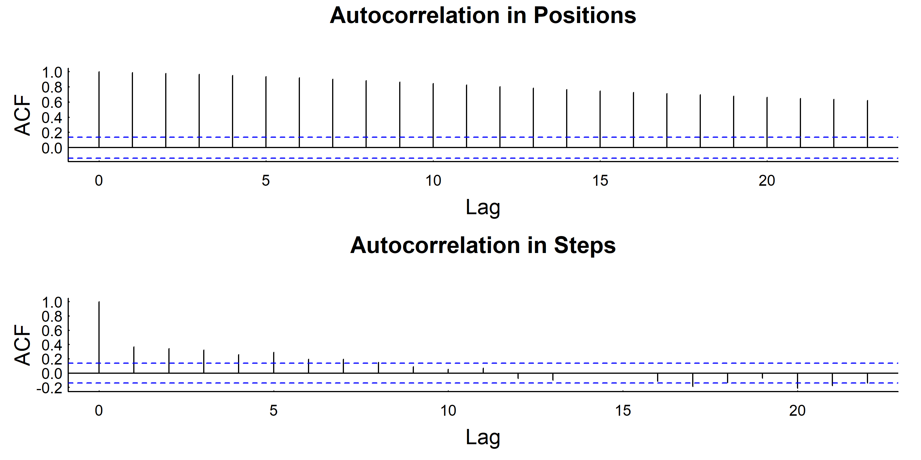
12.3.1 CRW Properties

# The CRW also shows autocorrelation in position
acf(Re(Z), main = "Autocorrelation in Positions")

# But NOT in the steps
acf(Re(diff(Z)), main = "Autocorrelation in Steps")

13 Multi-state Random Walk

Animals often switch between behavioral states (e.g., resting, foraging, traveling). We can model this using a Multi-state Random Walk where movement parameters depend on the behavioral state.

13.1 Markov Chains for State Transitions

First, we need to understand how to model state transitions using Markov chains. A Markov chain describes transitions between discrete states with fixed probabilities. We represent this with a transition probability matrix where element \(M_{ij}\) is the probability of transitioning from state \(i\) to state \(j\). The matrix has the structure:

\[\mathbf{M} = \begin{bmatrix} p_{11} & p_{12} & p_{13} \\ p_{21} & p_{22} & p_{23} \\ p_{31} & p_{32} & p_{33} \end{bmatrix}\]

where each element \(p_{ij} = P(X_{t+1} = j \mid X_t = i)\) represents the probability of transitioning from state \(i\) to state \(j\).

Note: because each row represents transition probabilities, their entries MUST sum to 1

\[\sum_{j=1}^{3} p_{ij} = 1 \quad \text{for all } i\]

If \(\boldsymbol{\pi}_t\) is a vector (list of numbers) representing the probability distribution over states at time \(t\):

\[\boldsymbol{\pi}_t = [\pi_1(t), \pi_2(t), \pi_3(t)]\]

then the distribution at the next time step is given by multiplying that vector my the transition matrix:

\[\boldsymbol{\pi}_{t+1} = \boldsymbol{\pi}_t \mathbf{M}\]

In component form:

\[\pi_j(t+1) = \sum_{i=1}^{3} \pi_i(t) \cdot p_{ij}\]

This says: the probability of being in state \(j\) at time \(t+1\) equals the sum over all states \(i\) of the probability of being in state \(i\) at time \(t\) times the probability of transitioning from \(i\) to \(j\).

Example: If we start with certainty in state 1, i.e., \(\boldsymbol{\pi}_0 = [1, 0, 0]\):

\[\boldsymbol{\pi}_1 = [1, 0, 0] \begin{bmatrix} 0.7 & 0.2 & 0.1 \\ 0.4 & 0.4 & 0.2 \\ 0.0 & 0.8 & 0.2 \end{bmatrix} = [0.7, 0.2, 0.1]\]

After one step, there’s a 70% chance of being in state 1, 20% in state 2, and 10% in state 3.

13.2 Simulating a Markov Chain

First, we specify the transition matrix. We’ll have 3 states, which we call “chilling” (state 1), “cruising” (state 2), and “huffing” (state 3), with the same matrix we described above.

M <- rbind(
  c(0.7, 0.2, 0.1),   # From chilling
  c(0.4, 0.4, 0.2),   # From cruising  
  c(0.0, 0.8, 0.2)    # From huffing
)

rownames(M) <- colnames(M) <- c("chilling", "cruising", "huffing")
M

         chilling cruising huffing
chilling      0.7      0.2     0.1
cruising      0.4      0.4     0.2
huffing       0.0      0.8     0.2

Let’s verify this is a valid transition matrix (rows sum to 1):

rowSums(M)

chilling cruising  huffing 
       1        1        1 

To simulate a sequence of states, at each time step you have to “sample” the transition probabilities for the fiven state. If you’re in staet 1, you sample from the first row of the matrix with the appropriate probabilities, if in row 2, you sample from the second row, etc:

n <- 400
states <- 1:3
State_mc <- rep(NA, n)  # empty simulation vector
State_mc[1] <- 1  # Start in "chilling" state

for(i in 2:n) {
  State_mc[i] <- sample(states, size = 1, prob = M[State_mc[i-1], ])
}

# Show first 100 states
State_mc[1:100]

  [1] 1 2 2 2 3 2 2 2 2 2 3 2 3 2 2 3 2 1 1 2 3 2 2 2 3 3 2 2 1 1 1 1 1 1 3 2 2
 [38] 3 3 2 3 2 2 2 3 2 1 3 2 2 2 2 1 2 1 2 3 2 3 2 2 2 1 2 1 1 1 2 3 2 3 2 1 1
 [75] 1 1 1 2 1 1 1 2 3 2 2 2 3 2 2 2 2 1 3 2 2 2 2 2 3 3

13.3 Calculate Stationary Distribution

The stationary distribution tells us the long-run proportion of time in each state. Empirically you just count percentages of time spent in each state:

table(State_mc) |> prop.table()

State_mc
   1    2    3 
0.48 0.36 0.16 

Mathematically, you can compute it directly from the transition probability using the “eigenvalue theorem” (see, e.g., this link). Long-story short, almost every square matrix is associated with a magic vector - the eigenvector \(({\bf v})\) and a magic number - the eigenvalue (\(\lambda\)) that satisfies the equation:

\[M \times {\bf v} = \lambda \times{\bf v}\]

which means: there is a set of numbers (e.g. a set of probabilities of being in a behavioral state), that - when you multiply the matrix magic to it - gives you the same vector, just multiplied by a factor.

13.4 Simulate Multi-state Random Walk

Now we’ll create a full multi-state random walk where movement parameters depend on the behavioral state.

# Movement parameters for each state
# State 1 (chilling): no persistence, small steps
# State 2 (cruising): medium persistence, medium steps  
# State 3 (huffing): high persistence, large steps

rhos <- c(0, 0.5, 0.9)        # turning angle concentration
alphas <- c(1, 2, 5)          # Weibull shape for step length
betas <- c(0.5, 3, 8)         # Weibull scale for step length

# Helper function for wrapped Cauchy
rwc <- function(n, mu, rho) {
  ifelse(rho == 0, 
         runif(length(rho == 0), 0, 2*pi), 
         rcauchy(n, mu, -log(rho)) %% (2 * pi))
}

# Simulate turning angles based on state
thetas <- rwc(n, mu = 0, rho = rhos[State_mc])

# Simulate step lengths based on state
step_lengths <- rweibull(n, shape = alphas[State_mc], scale = betas[State_mc])

# Create movement path
S <- complex(arg = cumsum(thetas), modulus = step_lengths)
Z <- cumsum(S)

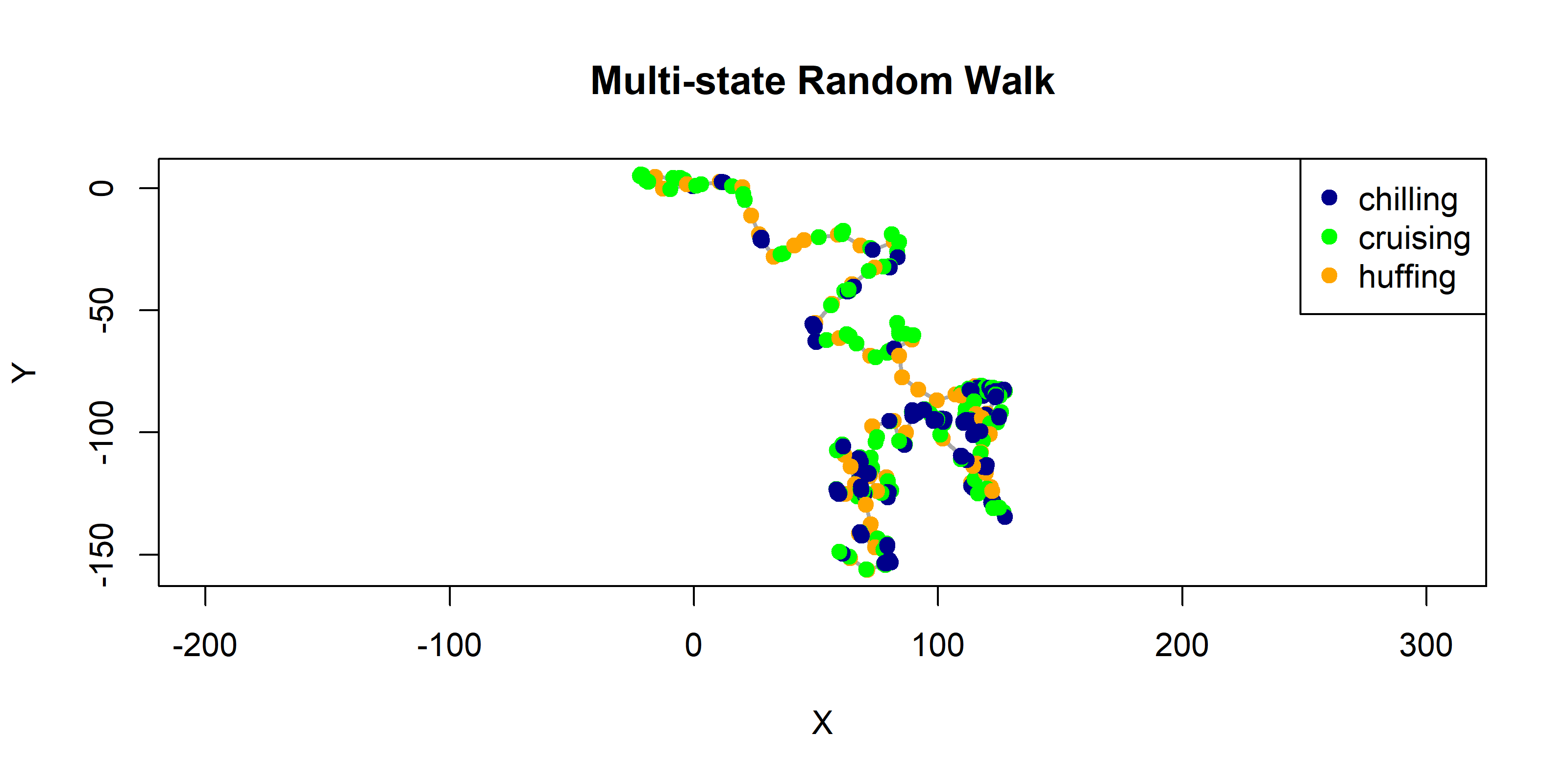
Visualize the multi-state random walk:

## pars()
cols <- c("darkblue", "green", "orange")
plot(Z, type = "l", col = "darkgrey", asp = 1, lwd = 2, 
     main = "Multi-state Random Walk", xlab = "X", ylab = "Y")
points(Z, col = cols[State_mc], pch = 19)
legend("topright", legend = rownames(M), col = cols, pch = 19)

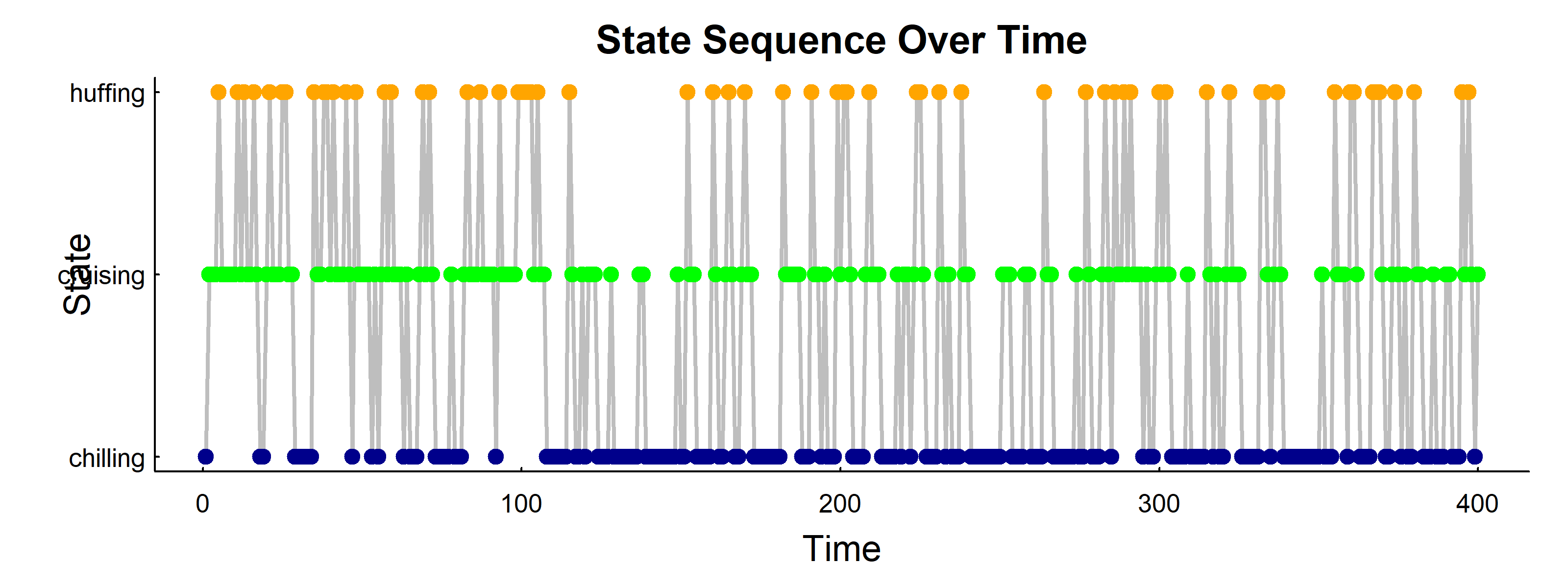
13.5 Visualize State Sequence

pars()
par(mar = c(3, 4, 2, 1))
plot(1:n, State_mc, type = "l", lwd = 2, col = "grey", 
     xlab = "Time", ylab = "State", yaxt = "n",
     main = "State Sequence Over Time")
points(1:n, State_mc, col = cols[State_mc], pch = 19)
axis(2, at = 1:3, labels = rownames(M), las = 1)

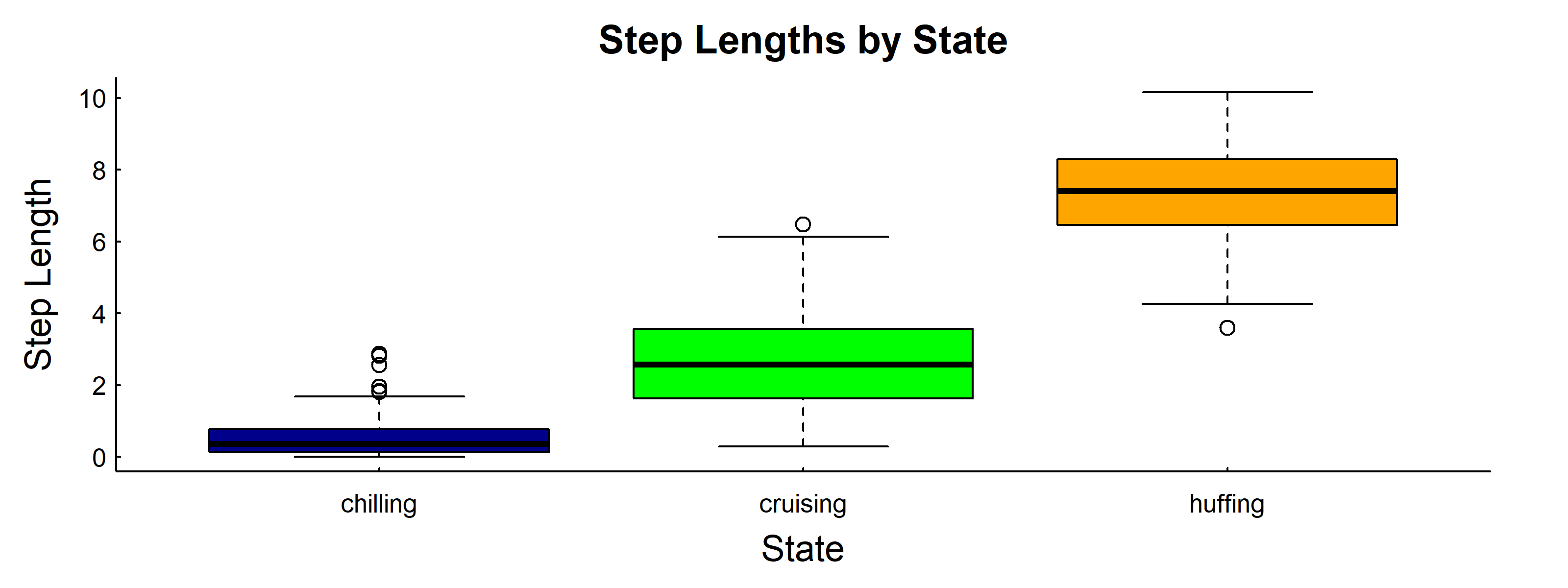
13.6 Compare Movement Parameters Across States

boxplot(step_lengths ~ State_mc, col = cols, 
        xlab = "State", ylab = "Step Length",
        names = rownames(M), main = "Step Lengths by State")

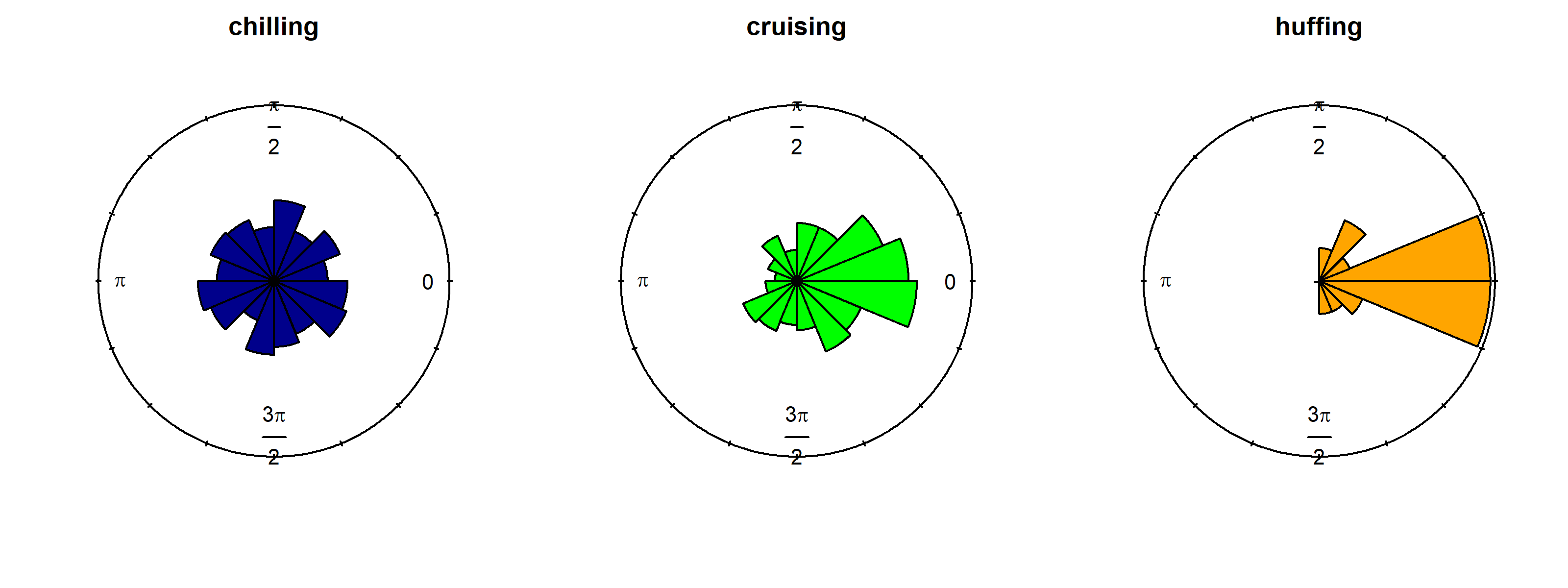
Note how I use a loop for the turning angles

require(circular)

for(i in 1:3)
rose.diag(thetas[State_mc == i], bins = 16, col = cols[i], 
          prop = 1.5, main = rownames(M)[i])

13.7 Some exercises

1. Random Walk Exploration: Simulate 1D and 2D random walks with different \(\sigma\) values. How does step size affect the area covered?

2. AR Process Behavior: Try different values of \(\phi\) (e.g., 0.3, 0.6, 0.9). How does this affect the home range size? Verify the home range formula.

3. CRW Persistence: Modify the rho parameter in the CRW. What happens when rho = 0 (no directional persistence) vs rho = 0.95 (high persistence)?

4. Multi-state Customization: Create your own transition matrix and movement parameters. Try modeling different behaviors like:

   • Migration (directional state with long steps)
   • Foraging (slow, tortuous movement)
   • Resting (minimal movement)

5. State Duration: Calculate the average duration animals spend in each state. Hint: Look at run lengths of consecutive states.

13.8 References

Kareiva, P. M., and N. Shigesada. 1983. “Analyzing Insect Movement as a Correlated Random Walk.” Oecologia 56: 234–38. https://doi.org/10.1007/BF00379695.

Patlak, C. S. 1953a. “A Mathematical Contribution to the Study of Orientation of Organisms.” Bulletin of Mathematical Biophysics 15: 431–76. https://doi.org/10.1007/BF02476435.

———. 1953b. “Random Walk with Persistence and External Bias.” Bulletin of Mathematical Biophysics 15: 311–38.