Figure 10.1: This painting is amazingly called Dash for Liberty, and reminds us that chicks are both highly individual, and capable of movement. (source: Wikimedia commons)
10.1 Some motivation
Way back in chapter Chapter 3, we argued that movement data was so complicated and fancy that we absolutely needed fancy statistical concepts just to wrap our modeling around the data. Somewhat dismissively, we contrasted movement data to the kind of experimental, design-based statistics that are usually summed up with ANOVA. And - in particular - we used an example of an experiment with the weights of chicks (Gallus gallus domesticus) as modeled against various diets. Very simple, controlled experimental design: A bunch of chicks, several diets, measure weights, apply ANOVA - and your simple questions, namely: what diet leads to larger chicks?, is immediately answered.
In fact, nothing is quite so simple. This chapter - which has nothing directly to do with spatial data or movement data - mainly serves to systematically illustrate via an example what mixed models (that combines fixed effects and random effects) actually are, and when and why we might choose to use them. It also illustrates a somewhat non-trivial, but very important, context for incorporating auto-correlation in a linear model. And all of that in the context of asking a very simple question, that emerges directly from a simple experimental design in a controlled experiment, namely: under what diet do chicks grow fastest?
10.2 Chick Weights
The data are located in all R installations, and called ChickWeight:
Note that the “-1” coerced all of the intercepts to 0. Also, all the effects are significant: Weight increases with Time on average at rate 6.85 g/day, some diets lead to a higher overall mean.
Pop quiz: What’s the difference between the following models? Which one matches the model above?
Chick.lm1<-lm(weight~Time*Diet, data =ChickWeight)Chick.lm2<-lm(weight~Time+Diet, data =ChickWeight)Chick.lm3<-lm(weight~Time:Diet, data =ChickWeight)
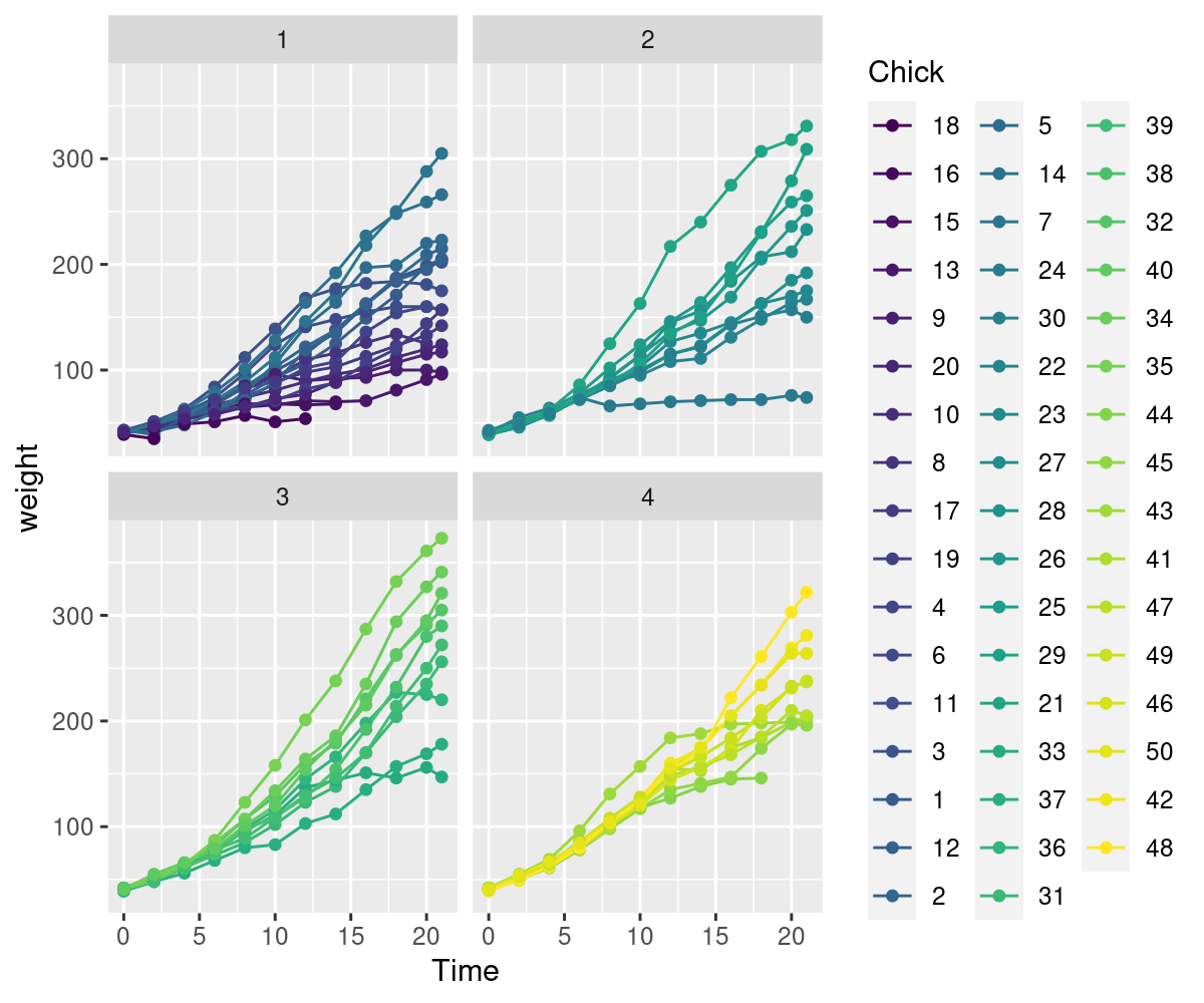
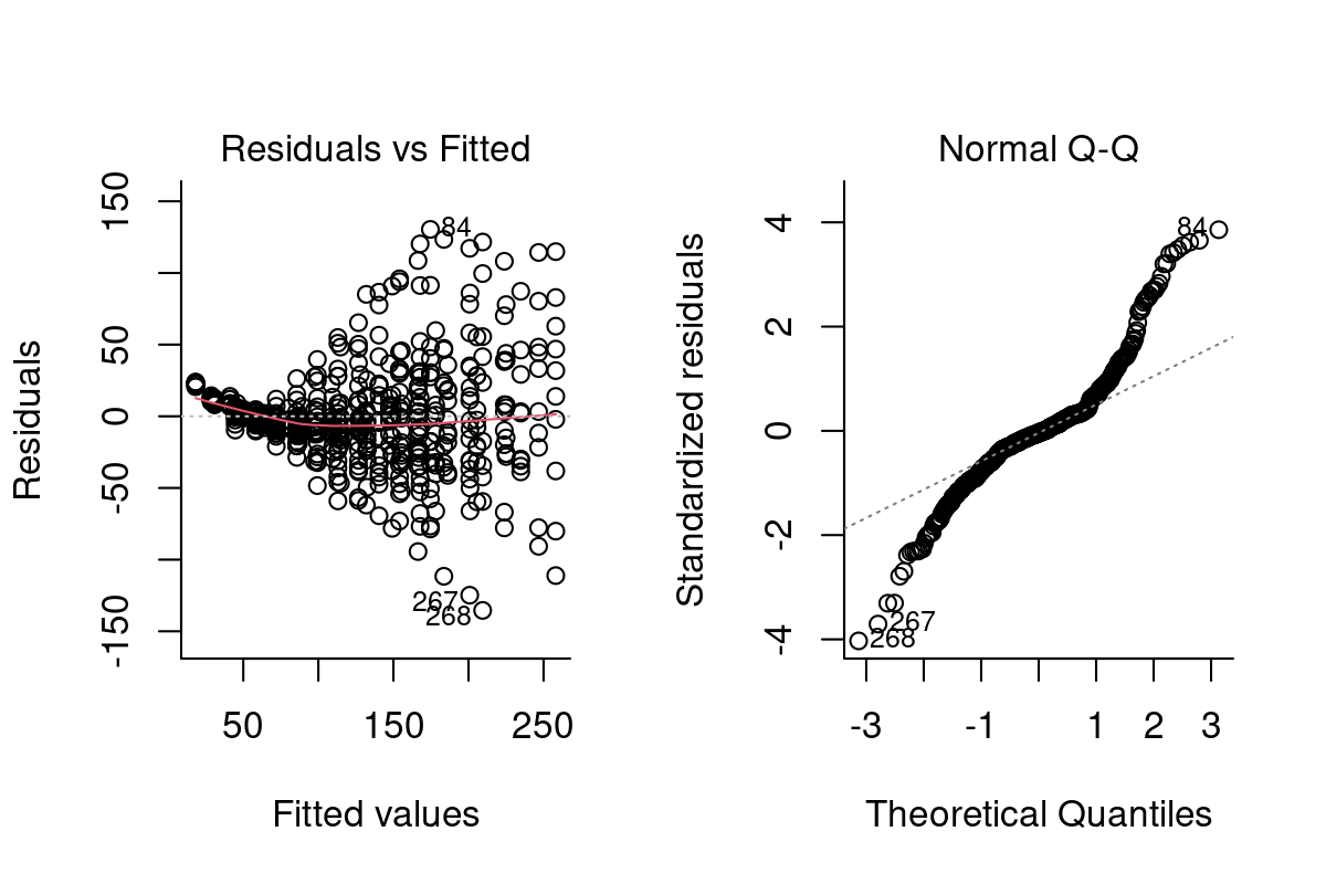
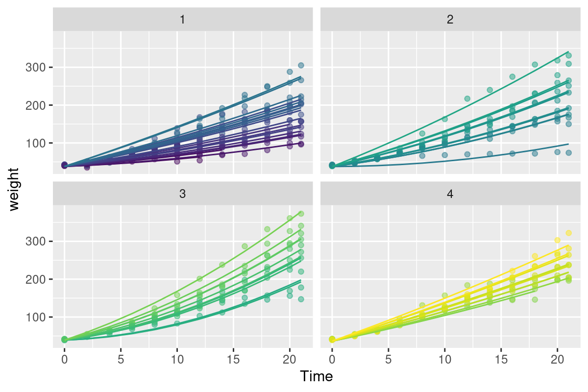
Both heteroskedasticity and kurtosis2 in the residuals are big problems. The main reason for that is that each individual bird is quite different from the others (see figure Figure 10.1).
2 Knock your socks off statsy vocab words!
10.3.2 Adding individual chicks
One option to deal with this is to simple include “individual bird” in the model:
Chick.lm2<-lm(weight~Time:Diet+Chick, data =ChickWeight)anova(Chick.lm2)
Analysis of Variance Table

Response: weight
           Df  Sum Sq Mean Sq F value    Pr(>F)
Chick      49  530105   10818  16.806 < 2.2e-16 ***
Time:Diet   4 2047136  511784 795.029 < 2.2e-16 ***
Residuals 524  337315     644
---
Signif. codes:  0 '***' 0.001 '**' 0.01 '*' 0.05 '.' 0.1 ' ' 1
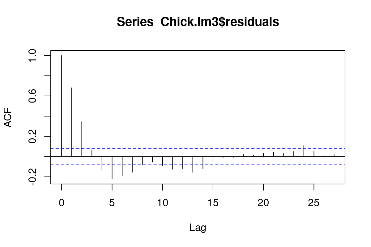
We’ve absorbed a lot of the variability, but there’s still strong structure to the residuals.
10.3.3 Individual slopes (and getting curvy)
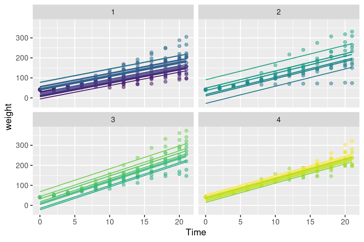
Somewhat better would be to let each individual have a unique slope as well. Let’s also not be naive, and a second order polynomial term to the model - because, you know, growth is not linear and all that:
Chick.lm3<-lm(weight~(Diet*poly(Time,2))+Time:(Chick-1), data =ChickWeight)anova(Chick.lm3)
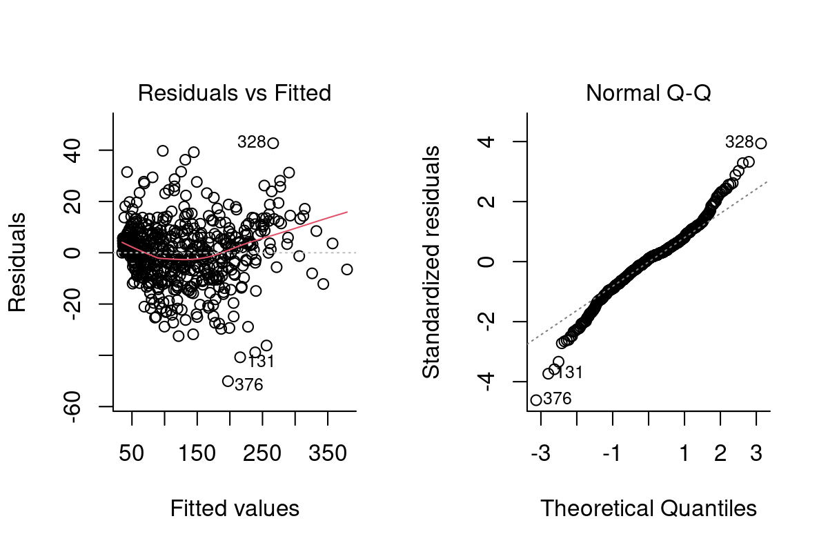
Well - this model is begginning to look mighty fine! Check out that astronomical R^2 (summary(Chick.lm3)$r.squared = 0.9929361) and decent looking residuals. The big problem, however, is that this has cost us ENORMOUS degrees of freedom! We’ve estimated length(Chick.lm3$coef) = 62 coefficients.
10.3.4 Quick comment on “updating”
Before we fix this problem, a quick comment on a “smarter” workflow for iteratively building models using the update function. This function basically takes your model and adds or removes features as desired.
For example, the Chick.lm1 model above was given by:
Chick.lm1$call
lm(formula = weight ~ Time * Diet, data = ChickWeight)
Whereas:
Chick.lm2$call
lm(formula = weight ~ Time:Diet + Chick, data = ChickWeight)
The update command lets you add additional structural elements, like correlations and random effects (as below), change the response variable, or change the data - without rewriting the entire model call.
10.4 Mixed effects models
The model fitted above looks something like this: \[Y_{ijk} = \alpha_i + (\beta_i + \kappa_j) T_{ijk} + \gamma_j T^2_{ijk} + \epsilon_{ij}\]
Where \(i \in \{1,2,3,4\}\) refers to diet, \(j \in {1,2, ..., 48}\) refers to individual chicken (each of which has a unique slope - but not intercept) and \(k\) to replicates.
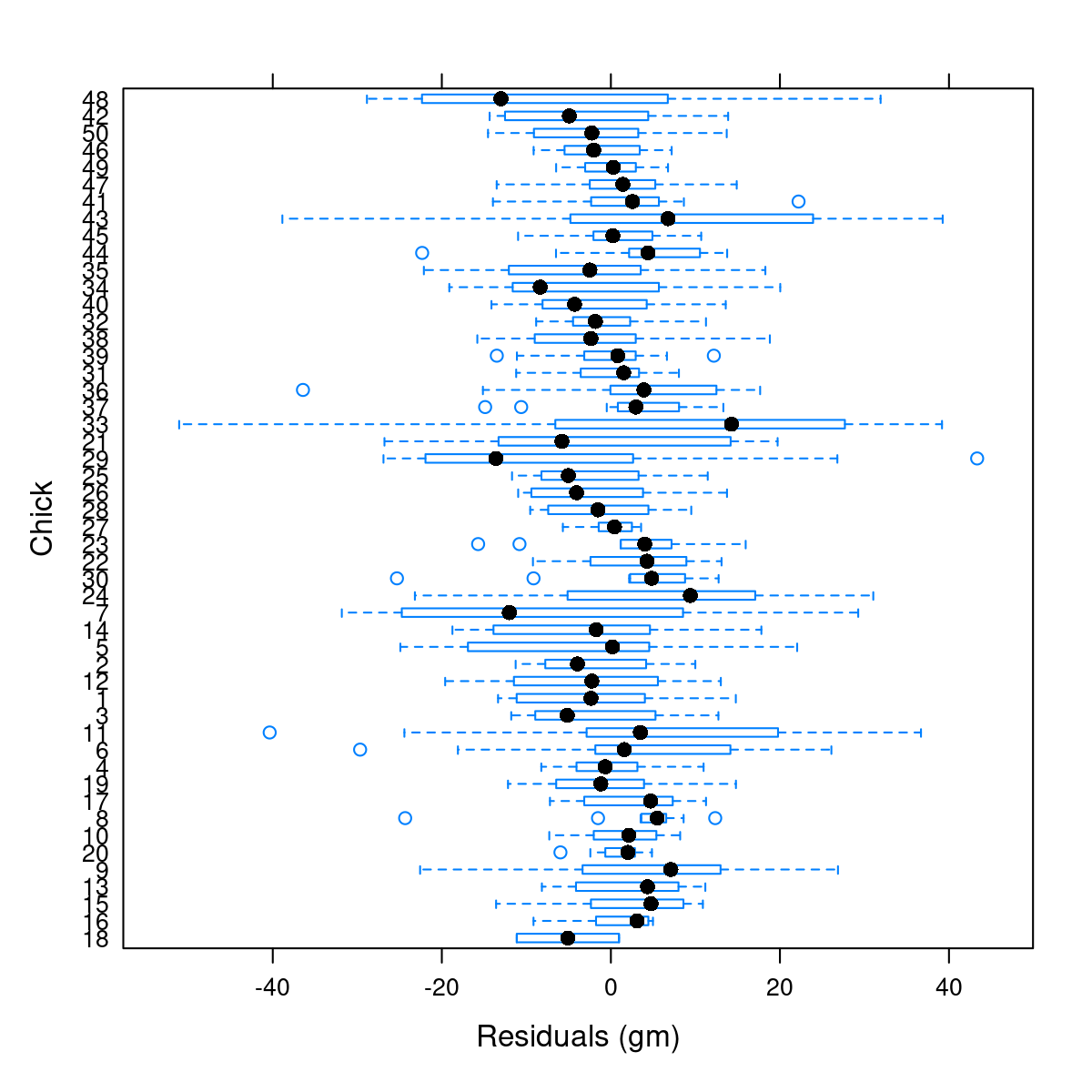
In fact, we don’t ACTUALLY care about individual birds! Wouldn’t it be great if we could take all of those \(\kappa_j\)’s and model them as a random variable? I.e.: \(\kappa_j \sim {\cal N}(\mu_\kappa, \sigma_\kappa)\)? Out of curiosity, lets look at all of the coefficients for the individual chicks:
That is exactly what a mixed effects model does! It’s called “mixed” because there are “fixed effects” (here, the diet, and the time are fixed effects, and the individual chick will be “random”).
where \(\beta\) is the (p-dimensional) vector of fixed effects \({\bf b}_i\) is the q-dimensional vector of random effects, \({\bf X}_i\) (\(n \times p\)) is a the known fixed effect regressor matrix, and \({\bf Z}_i\) (\(n \times q\)) is the random effects data matrix.
10.4.2 Applied to the chicks
The nlme package allows you to fit mixed effects models. So does lme4 - which is in some ways faster and more modern, but does NOT model heteroskedasticity or (!spoiler alert!) autocorrelation.
Let’s try a model that looks just like our best model above, but rather than have a unique Time slope for each chick, it will be a random variable. Thus: \[Y_{ijk} = \alpha_i + (\beta_i + K) T_{ijk} + \gamma_i T^2_{ijk} + \epsilon_{ij}\]
Where the slope on Time is given by the random parameter K, which has some distribution: \(K \sim {\cal N}(0, \sigma_k^2)\)
require(nlme)Chick.lme1<-lme(fixed =weight~Diet*poly(Time,2), random =~(Time-1)|Chick, data =ChickWeight, method ="ML")
The summary output of this function is massive … below a somewhat truncated version:
The following model adds 1st order autocorrelation to a 2nd order time model with a unique diet effect:
Chick.lme2<-lme(fixed =weight~Diet+poly(Time,2)-1, random =~(Time-1)|Chick, data =ChickWeight, correlation =corAR1())
Notice that the random grouping term is Time - 1 | Chick, i.e. the slopes for each chick is unique and modeled as a random variable, but the intercepts are always 0. Furthermore the intercept of the main effect variable is also set to 0 (via the -1). This makes sense biologically, but it is also the only way I could make a model with a serial autocorrelation converge.
This is - anyway - an excellent model. The summary:
Model selection based on AICc:

                            K    AICc Delta_AICc AICcWt Cum.Wt       LL
ChickModel.Diet.AutoCorr   15 4207.40       0.00      1      1 -2088.27
ChickModel.NoDiet.AutoCorr  9 4245.47      38.07      0      1 -2113.58
ChickModel.Diet            14 4790.13     582.73      0      1 -2380.69
ChickModel.NoDiet           8 4843.07     635.67      0      1 -2413.41
This is the commonly encountered delta AIC” table which sorts the models by increasing information criterion, and provides useful ancillary summaries. These tables are often reported in journal articles to provide support for model slection. Note that the function automatically chose the AICc (corrected AIC) as a criterion, which has better statistical properties for smaller sample sizes and lots of degrees of freedom. But the ultimate conclusion is the same.
10.5 Exercise: Does Diet Matter?
Summarize the conclusion of this analysis.
How many parameters are estimated in the “best” model? Report all of their values.
Expand the model selection to include models without the second order Diet term. Are any of those “better”.
Expand the model selection to include corresponding linear models, with individual chick fixed effects. How do they compare?


_(cropped).jpg)